63. The Hsieh-Clough-Tocher (HCT) elements#
According to Franco Brezzi, programming \(C^1\) continuous finite elements has the pleasure of Cod liver oil.
63.1. The problem with polynomial spaces#
Let us use the element space \(P^3\), and try to find dofs for a \(C^1\) conforming finite element space:
We need point values and the gradient in the vertices. This already fixes the whole function on the edge.
To obtain continuity of the normal derivative, we need an additional dof per edge
These are 12 dofs, but the dimension of \(P^3\) is only 10.
Increasing the order fron \(k\) to \(k+1\) does not help: Increasing the order by one adds \(O(k)\) \(C^1\)-bubbles, but only 2 functions per edge contributing to the trace and the normal derivative trace.
One way out is to use non-polynomial spaces.
63.2. The Alfeld split#
Insert a vetex \(V_c\) in the center of gravity of the traingle \(T\), and split \(T\) into 3 triangles \(t_1, t_2, t_3\) by connecting \(V_c\) with two of the original vertices. Then there is a space \(V_T\) such that
\(V_T\) is polynomial or order \(k \geq 3\)
\(V_T \subset C^1(T)\)
The degrees form above are unisolvent
One can implement such a finite element by choosing some polynomial basis on the sub-triangles, and implement the internal \(C^1\) constraints by additional equations. A more direct construction is possible by using a Bernstein basis
63.3. The Bernstein basis#
The Bernstein basis for polynomials of order \(n\) on the interval \(I=[0,1]\) is
where \(\lambda_0 = x\) and \(\lambda_1 = 1-x\). The nice thing is that the derivative can be expressed as a sum of two Bernstein basis polynomials of one order less:
The Bernstein basis on triangles (and higher dimensional simplices) is given by
This basis functions can be associated to nodes \(x_{ijk} = \sum_{m=1}^3 \lambda_i V_i\)
The directional derivative in direction \(d\) (with the \(m^{th}\) unit-vector \(e_m\)) is
i.e. it can be expressed by a small number of basis functions.
63.4. HCT triangle and the Bernstein basis:#
Consider a piecewise \(P^3\) basis function. On every sub-triangle we use the Bernstein basis, the coefficients are associated with the nodes:
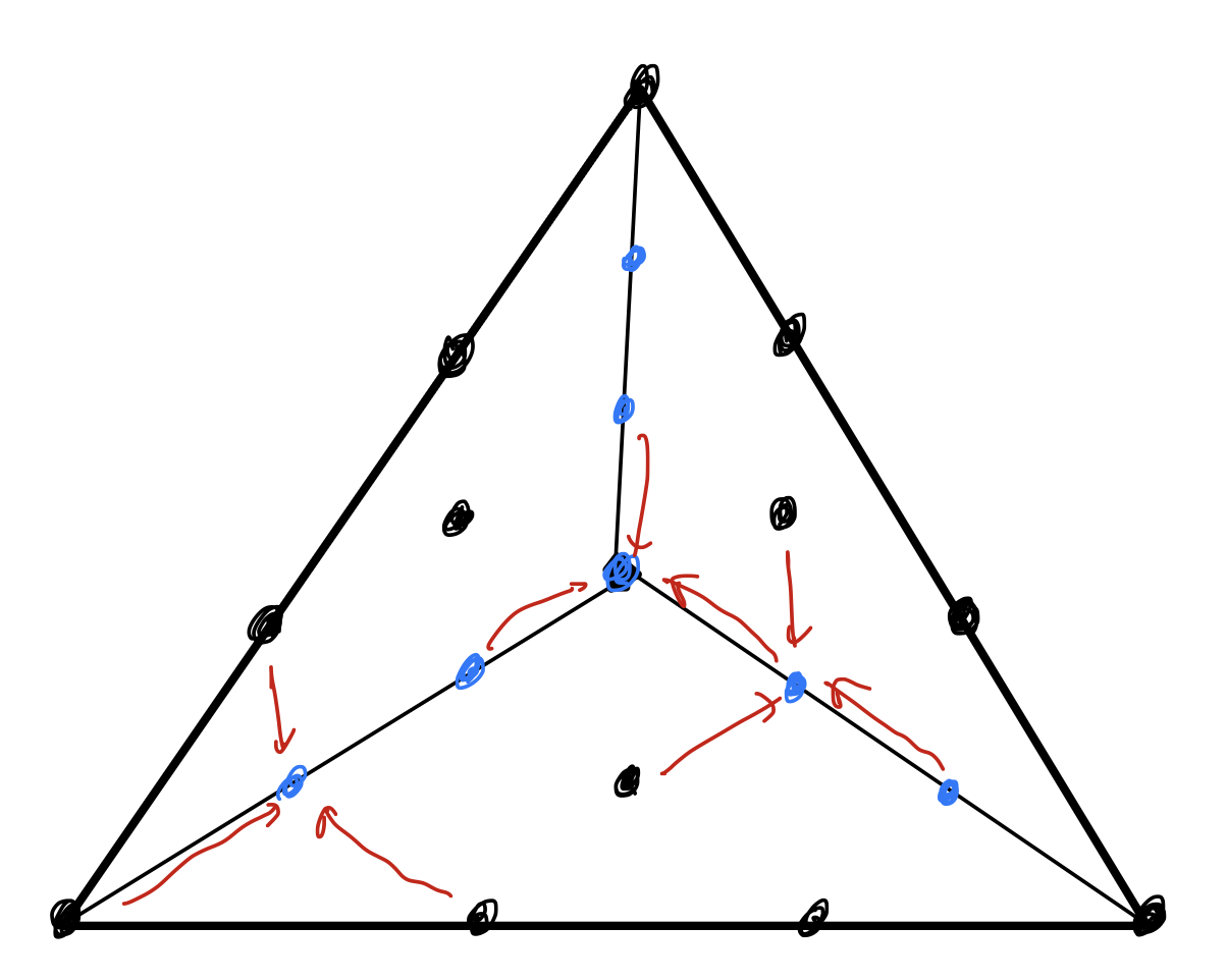
As with Lagrange elements, the trace of a function on the edge is given by the values in the nodes on the edge. Thus, \(C^0\)-continuity is obtained by the placement of the nodes. Since the derivatives of every Bernstein polynomial are expressed by only 3 polynomials, the \(C^1\) constraint envolves only nodes close to the edges.
Elementary but technical calculations lead to a very simple result: If the coefficients associated with the blue nodes are the arithmetic mean of the surrounding nodes as drawn by the red arrows, the function on the macro element is \(C^1\). The values in the black nodes are independent coefficients.
Comaring the \(P^3\) HCT element to the \(P^3\) Lagrange element, we see the function trace coincide, but the HCT element has more internal dofs. These allow to satisfy the continuity constraint along edges.
63.5. HCT in NGSolve#
The space HCT_FESpace is available With NGSolve 6.2.2603. It provides \(C^0\)-continuous finite elements, which allow to enforce \(C^1\)-continuity by Lagrange parameters:
elements space is \(P^k\) on the sub-triangles
continuity of the normal derivative along edges is enforced by a Lagrange parameter of order \(k-1\).
Since these constraints are not linearly independent, the resulting system would be singular, and thus a small regularization must be added.
from ngsolve import *
from netgen.occ import *
from ngsolve.webgui import Draw
mesh = Mesh(unit_square.GenerateMesh(maxh=0.1))
# mesh = Circle((0,0),1).Face().GenerateMesh(maxh=0.2, dim=2).Curve(3)
Draw (mesh);
order = 4
fes = HCT_FESpace(mesh, order=order, dirichlet=".*")
feslam = FacetFESpace(mesh, order=order-1)
X = fes*feslam

irs = fes.GetIntegrationRules()
n = specialcf.normal(2)
(u,lam),(v,mu) = X.TnT()

bfa = BilinearForm(X)
bfa += InnerProduct (u.Operator("hesse"), v.Operator("hesse"))*dx(intrules=irs)
bfa += (grad(u)*n*mu+ grad(v)*n*lam) * dx(element_boundary=True, bonus_intorder=3)
bfa += -1e-8 * lam*mu* dx(element_boundary=True)
bfa.Assemble()
lff = LinearForm(1000*v*dx(intrules=irs)).Assemble()
inv = bfa.mat.Inverse(freedofs=X.FreeDofs())
gfu = GridFunction(X)
gfu.vec.data = inv * lff.vec

gfuu = gfu.components[0]
Draw (gfuu, mesh);
Draw (grad(gfuu), mesh)
Draw (gfuu.Operator("hesse")[0,0], mesh);