60. Preconditioning

We call \(C\) a preconditioner to the matrix \(A\) if

• \(C^{-1} A \approx I\)

• the matrix-vector multiplication \(w = C^{-1} r\) is cheap

One extreme case is \(C = A\), where the first goal is optimally satisfied, but (in general) not the second. The opposite extreme is \(C = I\).

If \(A\) is an SPD matrix, we like to have an SPD preconditioner \(C\). In this case, the quality of the approximation can be measured by the spectral bounds

\[ 0 < \gamma_1 \leq \frac{x^T A x }{x^T C x} \leq \gamma_2 \qquad \forall \, 0 \neq x \in {\mathbb R^n} \]

The Rayleigh quotient is bounded by \(\gamma_1\) and \(\gamma_2\) from below and from above. These spectral bounds are bounds for the eigenvalues \(\lambda\) of the generalized eigenvalue problem

\[ A x = \lambda C x \]

If \(\lambda_i\) is an eigenvalue with eigenvector \(x_i\), then \(x_i^T A x_i = \lambda_i x_i^T C x_i\), and thus \(\lambda_i \in [\gamma_1, \gamma_2]\).

60.1. The preconditioned Richardson iteration

We use the preconditioner to obtain the correction from the residuum:

\[ \qquad x^{k+1} = x^k + \alpha C^{-1} (b - A x^k) \]

The error is now propagated as

\[ e^{k+1} = M e^k = (I - \alpha C^{-1} A) e^k \]

If we could use the ideal preconditioner \(C = A\), and set \(\alpha = 1\), then \(M = 0\), and we converge in one iteration.

The error-propagation matrix \(M\) is self-adjoint in the energy inner product

\[\begin{align*} \left< M x, y \right>_A &= (A M x)^T y \\ & = \left\{ A (x - \alpha C^{-1} A x) \right\}^T y \\ & = x^T (A - \alpha A C^{-1} A) y \\ & = \left< x, M y \right>_A \end{align*}\]

as well as in the inner products

\[ \left< x, y \right>_C \qquad \text{and} \qquad \left< x, y \right>_{AC^{-1} A}. \]

The error is monotonically decreased in the corresponding norms. In particular the last one is practically interesting since it is computationally available:

\[\begin{eqnarray*} \| x - x^\ast \|_{AC^{-1} A}^2 & = & \| A (x - x^\ast) \|_{C^{-1}}^2 \\ & = & \| A x - b \|_{C^{-1}}^2 \end{eqnarray*}\]

With the residuum \(r\) and preconditioned residuum \(w\), i.e.

\[ r = b - A x \qquad \text{and} \qquad w = C^{-1} r \]

the error becomes

\[ \| x - x^\ast \|_{AC^{-1}A}^2 = r^T w \]

from ngsolve import *
mesh = Mesh(unit_square.GenerateMesh(maxh=0.1))
fes = H1(mesh, order=1)
u,v = fes.TnT()
a = BilinearForm(grad(u)*grad(v)*dx+10*u*v*dx).Assemble()
f = LinearForm(x*y*v*dx).Assemble()
gfu = GridFunction(fes)

A very simple preconditioner is the Jacobi-preconditioner

\[ C = \text{diag} A \]

If \(A\) is SPD, then all diagonal entries are positive, and \(C\) is SPD as well.

In NGSolve, we can obtain a Jacobi preconditioner as follows:

pre = a.mat.CreateSmoother()

The result is a linear operator pre providing the linear operation

\[ w := C^{-1} * r \]

preforming the vector iteration to obtain the largest eigenvalue of \(C^{-1} A\):

hv = gfu.vec.CreateVector()
hv2 = gfu.vec.CreateVector()
hv3 = gfu.vec.CreateVector()
hv.SetRandom()
hv.data /= Norm(hv)
for k in range(20):
    hv2.data = a.mat * hv
    hv3.data = pre * hv2
    rho = Norm(hv3)
    print (rho)
    hv.data = 1/rho * hv3

0.5628463859901822
1.3004844587339315
1.3642450612653385
1.4017278282832695
1.428927912054942
1.451197927296262
1.4709697187344926
1.489456390475471
1.5072557909082451
1.5246072026789994
1.5415208146951107
1.5578609944298918
1.5734139487420609
1.587947333438726
1.6012589050513686
1.613209024712011
1.6237346368041081
1.632846787976177
1.6406169867162068
1.6471585575973842

Run the preconditioned Richardson iteration with diagonal preconditioning:

alpha = 1 / rho
r = f.vec.CreateVector()
w = f.vec.CreateVector()
gfu.vec[:] = 0

w.data = pre * f.vec
err0 = sqrt(InnerProduct(f.vec, w))
its = 0
errhist = []
while True:
    r.data = f.vec - a.mat * gfu.vec
    w.data = pre * r
    err = sqrt(InnerProduct(r,w))
    # print ("iteration", its, "res=", err)
    errhist.append (err)
    gfu.vec.data += alpha * w
    if err < 1e-8 * err0 or its > 10000: break
    its = its+1
print ("needed", its, "iterations")

needed 1234 iterations

import matplotlib.pyplot as plt
plt.yscale('log')
plt.plot (errhist);

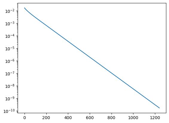
By situation is not considerably improved by the diagonal preconditioner. However, if we have a bilinear-form with variable coefficient, or large coefficients in the Robin - boundary condition such as

\[ A(u,v) = \int_\Omega \nabla u \nabla v \, dx + 10^8 \int_{\Gamma_R} u v \, ds, \]

the Jacobi preconditioner captures these parameters (experiment in excercise, theory soon).

60.2. The preconditioned gradient method

To introduce the preconditioner into the gradient method we proceed as follows. Since \(C\) is SPD, we are allowed to form its square-root

\[ C^{1/2} \]

as well as its inverse. The linear system \(A x = b\) is equivalent to

\[ C^{-1/2} A C^{-1/2} \; C^{1/2} x = C^{-1/2} b. \]

With the definition of transformed quantities

\[ \tilde A = C^{-1/2} A C^{-1/2}, \qquad \tilde b = C^{-1/2} b, \qquad \tilde x = C^{1/2} x \]

we have the linear system

\[ \tilde A \tilde x = \tilde b. \]

The transformed matrix \(\tilde A\) is SPD as well.

We apply the gradient method for the transformed system:

Given \(\tilde x^0\)
\(\tilde r^0 = \tilde b - \tilde A \tilde x^0\)
for \(k = 0, 1, 2, \ldots\)
\(\qquad \tilde p = \tilde A \tilde r^k\)
\(\qquad \alpha = \frac{{\tilde r^k}^T \tilde r^k }{ {\tilde r^k}^T \tilde p}\)
\(\qquad \tilde x^{k+1} = \tilde x^k + \alpha \tilde r^k\)
\(\qquad \tilde r^{k+1} = \tilde r^k - \alpha \tilde p\)

The error analysis of the gradient method provides

\[ \| \tilde x^\ast - \tilde x^{k+1} \|_{\tilde A} \leq \rho \| \tilde x^\ast - \tilde x^{k} \|_{\tilde A}, \]

and substituting back

\[ \| x^\ast - x^{k+1} \|_A \leq \rho \| x^\ast - x^{k} \|_A \]

Since we cannot compute with the transformed system we transform back via

\[ \tilde x^k = C^{1/2} x^k, \qquad \tilde r^k = C^{-1/2} r, \qquad \tilde p = C^{-1/2} p \]

and obtain

Given \(x^0\)
\(C^{-1/2} r^0 = C^{-1/2} b - C^{-1/2} A C^{-1/2} C^{1/2} x^0\)
for \(k = 0, 1, 2, \ldots\)
\(\qquad C^{-1/2} p = C^{-1/2} A C^{-1/2} C^{-1/2} r^k\)
\(\qquad \alpha = \frac{\{C^{-1/2} r^k \}^T C^{-1/2} r^k \, }{ \, \{ C^{-1/2} r^k\}^T C^{-1/2} p}\)
\(\qquad C^{1/2} x^{k+1} = C^{1/2} x^k + \alpha C^{-1/2} r^k\)
\(\qquad C^{-1/2} r^{k+1} = C^{-1/2} r^k - \alpha C^{-1/2} p\)

now we simplify, and introduce \(w = C^{-1} r\)

Given \(x^0\)
\(r^0 = b - A x^0\)
for \(k = 0, 1, 2, \ldots\)
\(\qquad w = C^{-1} r^k\)
\(\qquad p = A w\)
\(\qquad \alpha = \frac{w^T r^k}{w^T p^k}\)
\(\qquad x^{k+1} = x^k + \alpha w\)
\(\qquad r^{k+1} = r^k - \alpha p\)

r = f.vec.CreateVector()
w = f.vec.CreateVector()
p = f.vec.CreateVector()

gfu.vec[:] = 0
r.data = f.vec
w.data = pre*r
err0 = sqrt(InnerProduct(r,w))
its = 0
errhist = []
while True:
    w.data = pre*r
    p.data = a.mat * w
    err2 = InnerProduct(w,r)
    alpha = err2 / InnerProduct(w,p)

    # print ("iteration", its, "res=", sqrt(err2))
    errhist.append (sqrt(err2))
    gfu.vec.data += alpha * w
    r.data -= alpha * p
    if sqrt(err2) < 1e-8 * err0 or its > 10000: break
    its = its+1
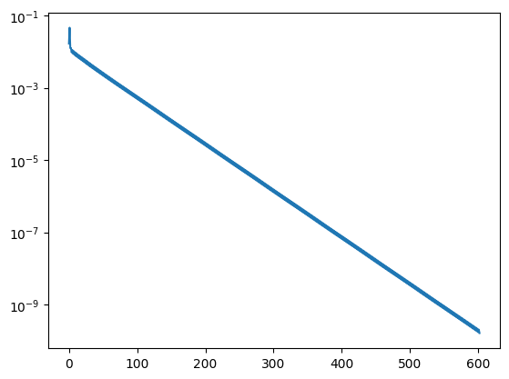
print ("needed", its, "iterations")

needed 602 iterations

plt.yscale('log')
plt.plot(errhist);

60.3. Jacobi and Gauss Seidel Preconditioners

For a given residual \(r\), the Jacobi preconditioner computes

\[ w = D^{-1} r \]

with \(D = \text{diag} A\). If \(r_i\) is the \(i^{th}\) component of the residual, the correction step of the \(i^{th}\) variable is \(w_i = A_{ii}^{-1} r_i\). All these correction steps are computed for the same residual.

In contrast, the Gauss-Seidel iteration updates the \(i^{th}\) variable from the residual computed from all up to date variables:

for \(i = 1, \ldots, n\):
\(\qquad \hat x_i = x_i + A_{ii}^{-1} \big( b_i - \sum_{j=1}^{i-1} A_{ij} \hat x_j - \sum_{j=i}^n A_{ij} x_j \big)\)

The method depends on the enumeration of variables. E.g, one could loop backwards, and thus obtains the so-called backward Gauss-Seidel iteration.

There holds for every \(1 \leq i \leq n\): $\( \sum_{j=1}^i A_{ij} \hat x_j = b_i - \sum_{j=i+1}^n A_{ij} x_j \)$

If we split the matrix

\[ A = L + D + R \]

with a strictly lower triangular matrix \(L\), a diagonal matrix \(D\), and a strictly upper diagonal matrix \(R\) we can write

\[ (L+D) \hat x = b - R x \]

or

\[ (L+D) \hat x = (L+D) x + b - A x \]

or

\[ \hat x = x + (L+D)^{-1} (b - A x) \]

This means we can interpret the Gauss-Seidel iteration as a preconditioned Richardson iteration, with preconditioner \(C = L+D\). In general, this is not a symmetric preconditioner.

If we run the backward Gauss-Seidel iteration, the preconditioner becomes \(C = D + R\). Now, we combine one step forward, with one step backward Gauss-Seidel:

\[\begin{eqnarray*} \tilde x & = & x + (L+D)^{-1} (b - A x) \\ \hat x & = & \tilde x + (D+R)^{-1} (b - A \tilde x) \end{eqnarray*}\]

we can rewrite it as

\[\begin{eqnarray*} \hat x & = & (D+R)^{-1} (b - L \tilde x) \\ & = & (D+R)^{-1} \big(b - L (L+D)^{-1} (b - R x) \big) \\ & = & (D+R)^{-1} \big( (L+D)(L+D)^{-1} b - L (L+D)^{-1} b \big) + \ldots x \\ & = & (D+R)^{-1} D (L+D)^{-1} b + \ldots x \\ & = & x + (D+R)^{-1} D (L+D)^{-1} (b - A x) \end{eqnarray*}\]

and observe that the combined forward-backward Gauss-Seidel iteration is a Richardson method with preconditioner

\[ C_{FBGS}^{-1} = (D+R)^{-1} D (L+D)^{-1}. \]

If \(A\) is symmetric, then \((L+D)^T = D+R\), and \(C_{FBGS}\) is symmetric as well. If \(A\) is SPD, then we obtain

\[ x^T C_{FBGS} x \geq x^T A x \qquad \forall \, x \]

i.e. the spectral constant \(\gamma_2 = 1\), and choosing a damping parameter \(\alpha = 1\) is guaranteed to converge.

We prove this by calculation:

\[\begin{eqnarray*} C_{FBGS} & = & (L+D) D^{-1} (D+R) \\ & = & L + D + R + L D^{-1} R \\ & = & A + L D^{-1} R \end{eqnarray*}\]

Since \(x^T L D^{-1} R x = (R x)^T D^{-1} (R x) = \| R x \|_{D^{-1}}^2 \geq 0\) we have proven that

\[ C_{FBGS} \geq A \]

The error propagation matrix of the FB - GS is

\[ M_{FBGS} = \underbrace{(I - (D+R)^{-1} A)}_{M_{BGS}} \underbrace{ ( I - (D+L)^{-1} A) }_{M_{FBS}}, \]

and has norm \(\| M_{FBGS} \|_A < 1\). The error propagation matrices of the forward GS and the backward GS are \(A\)-adjoint to each other:

\[ \left< M_{FGS} x, y \right>_A = \left< x, M_{BGS} y \right>_A \]

Thus, a single forward (or single backward Gauss-Seidel) step is also convergenct:

\[ \left< M_{FGS} x, M_{FGS} x \right>_A = \left< M_{BGS} M_{FGS} x, x \right>_A \leq \| M_{FBGS} \|_A \| x \|_A^2 \]

Exercise: Repeat the experiments with the forward-backward Gauss-Seidel preconditioner. You get it via pre = a.mat.CreateSmoother(GS=True). What do you observe for the spectral radius of \(C^{-1} A\) ?