18. Experiments with norms

We numerically compute the coefficients \(c_1, c_2 \in {\mathbb R}^+\) of equivalent norms

\[ c_1 \, \| u \|_B^2 \leq \| u \|_A^2 \leq c_2 \, \| u \|_B^2 \qquad \forall \, u \in V. \]

We assume that both norms are generated by inner products, i.e. \(\| u \|_A^2 = A(u,u)\) and \(\| u \|_B^2 = B(u,u)\).

To perform computations we need finite dimensional spaces. For function spaces \(V\), we choose finite element sub-spaces of mesh-size \(h\) and polynomial order \(p\). We compute on a sequence of spaces \(V_{h,p}\), to obtain \(c_1(h,p)\) and \(c_2(h,p)\). If these functions \(c_1\) and \(c_2\) seem to be bounded uniformly in \(h\) and \(p\), there is hope that the norm equivalence holds true also on the Sobolev space \(V\). This does NOT replace a mathematical analysis, but may help to decide if it is worth spending time to prove the estimate, or better search for a counter example.

By means of a basis for \(V_h\), we can rewrite the norm equivalence in \({\mathbb R}^N\) with \(N = \operatorname{dim} \, V_h\)

\[ c_1 \, u^T B u \leq u^T A u \leq c_2 u^T B u \qquad \forall \, u \in {\mathbb R}^N, \]

with representation matrices \(A\) and \(B\), or also with lower and upper bounds for the Rayleigh quotient

\[ c_1 \leq \frac{u^T A u}{u^T B u} \leq c_2 \qquad \forall \, u \in {\mathbb R}^N, \; u \neq 0 \]

Stationary points of the Rayleigh quotient are eigenvectors of the generalized eigenvalue-problem: find \(\lambda \in {\mathbb R}\) and \(u \in {\mathbb R}^N\) such that

\[ A u = \lambda B u. \]

The eigenvalues \(\lambda\) are the values of the quotient. In particular, the smallest and largest eigenvalues give sharp bounds for \(c_1\) and \(c_2\).

NGSolve provides the solver LOBPCG to compute a small number \(m\) of eigenpairs corresponding to the smallest \(m\), or largest \(m\) eigenvalues. Both matrices must by symmetric, and \(B\) must be also positive definite.

Note: The option for the largest eigenvalues was added 2024-03-16 (can use pip install --upgrade --pre ngsolve). For prior versions you have to swap the matrices \(A\) and \(B\), search for the smallest eigenvalue, and replace \(\lambda\) by \(1/\lambda\).

from ngsolve import *
from netgen.occ import *
from ngsolve.webgui import Draw
import matplotlib.pyplot as plt

18.1. Friedrichs’ inequality

We want to find a sharp constant \(c_F\) in Friedrich’s inequality $\( \| u \|_{L_2} \leq c_F \| \nabla u \|_{L_2} \quad \forall \, v \in H_{0,D}^1(\Omega), \)\( with \)\Omega = (0,1)^2$, and Dirichlet on the left and on the right side of the domain.

\[ c_F^2 = \sup_{u \in H_{0,D}^1} \frac{\| u \|_{L_2}^2}{ \| \nabla u \|_{L_2}^2 } \]

def SetupProblem(h,p):
    mesh = Mesh(unit_square.GenerateMesh(maxh=h))
    fes = H1(mesh, order=p, dirichlet="left|right")
    u,v = fes.TnT()
    L2Norm = BilinearForm(u*v*dx).Assemble().mat
    H1SemiNorm = BilinearForm(grad(u)*grad(v)*dx).Assemble().mat
    pre = Projector(fes.FreeDofs(), range=True)
    return L2Norm, H1SemiNorm, pre, fes

A,B,P,fes = SetupProblem(0.1, 5)
evals,evecs = solvers.LOBPCG(A, B, pre=P, num=5, maxit=200, largest=True, printrates=False)
print ("eigenvalues: ", list(evals))
print ("Friedrichs' constant: c_F = ", sqrt(evals[-1]))
print ("inverse of Friedrichs' constant: 1/c_F = ", 1/sqrt(evals[-1]))

gfu = GridFunction(fes)
gfu.vec.data = evecs[-1]
gfu.vec.data  /= Integrate(gfu*dx, fes.mesh) # normalize eigenfunction

eigenvalues:  [0.020264232604018606, 0.020264234576601235, 0.025330291735910584, 0.05066057588433867, 0.10132093820158772]
Friedrichs' constant: c_F =  0.31830950064612856
inverse of Friedrichs' constant: 1/c_F =  3.1415964586986087

Draw (gfu);

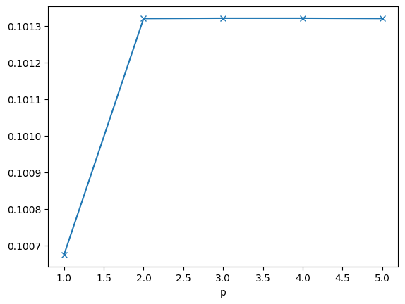
We compute on a sequence of spaces, and observe that the maximal eigenvalue converges very fast. This is in agreement to Friedrichs’ inequality which we have proven above.

lams = []
for p in range(1,6):
    A,B,P,fes = SetupProblem(0.1, p)
    evals,evecs = solvers.LOBPCG(A, B, pre=P, num=5, maxit=200, largest=True, printrates=False)
    lams.append([p,evals[-1]])

print (lams)
plt.xlabel("p")
plt.plot(*zip(*lams), '-x');

[[1, 0.10066207816841645], [2, 0.10132037983620129], [3, 0.10132118307694862], [4, 0.1013211807015426], [5, 0.10132105302197744]]

18.1.1. Inverse estimates

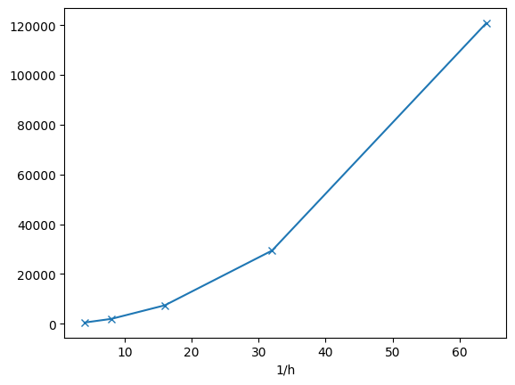
Now we search for the other bound for the norm equivalence, i.e.

\[ \| \nabla u_h \|_{L_2(\Omega)} \leq c(h,p) \, \| u_h \|_{L_2(\Omega)} \qquad \forall \, u_h \in V_{hp}, \]

where the (squared) sharp bound is the maximizer of the Rayleigh quotient

\[ c(h,p)^2 = \sup_{u \in V_{hp}} \frac{\|\nabla u\|^2_{L_2}}{\|u\|_{L_2}^2} \]

lams = []
for level in range(2,7):
    h = 0.5**level
    A,B,P,fes = SetupProblem(h, 1)
    evals,evecs = solvers.LOBPCG(B, A, pre=P, num=5, maxit=200, printrates=False, largest=True)
    lams.append([1/h,evals[-1]])

print (lams)
plt.xlabel("1/h")
plt.plot(*zip(*lams), '-x');

[[4.0, 501.7907346494362], [8.0, 2135.562283477553], [16.0, 7804.143924722657], [32.0, 34633.518845029685], [64.0, 133659.6480462116]]

lammins = []
for p in range(1,6):
    A,B,P,fes = SetupProblem(0.2, p)
    evals,evecs = solvers.LOBPCG(B, A, pre=P, num=5, maxit=200, printrates=False, largest=True)
    lammins.append([p,evals[-1]])

print (lammins)
plt.xlabel("p")
plt.plot(*zip(*lammins), '-x');

[[1, 653.1789330005993], [2, 3530.0518600005494], [3, 8675.114305718318], [4, 16992.87607688173], [5, 23725.095680466304]]

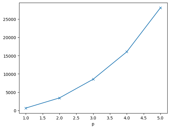
We clearly see that now the largest eigen-values grow as we refine the mesh, or increase the order. On every finite dimensional space the estimate \(\| \nabla u \|_{L_2} \leq c \| u \|_{L_2}\), but the constant grows with \(1/h\) and \(p\). This is called an inverse estimate.

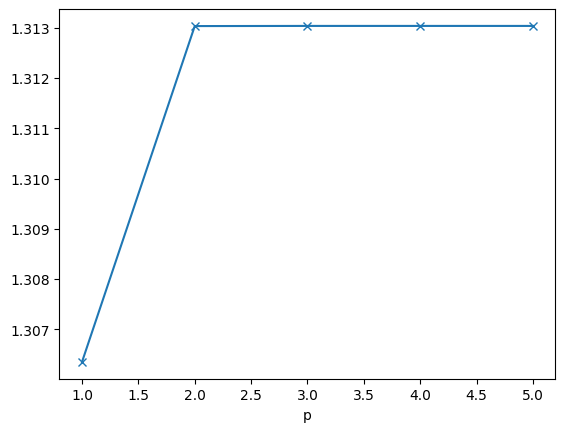
18.2. Trace inequality

We have proven there exists a continuous trace operator \(\operatorname{tr} H^1(\Omega) \rightarrow L_2(\partial \Omega)\), its norm is

\[ \| \operatorname{tr} \|^2 = \sup_{u \in H^1} \frac{\| \operatorname{tr} u \|_{L_2(\Gamma_D)}^2} {\|u\|_{H^1}^2} \]

We verify this numerically:

def SetupTraceProblem(h,p):
    mesh = Mesh(unit_square.GenerateMesh(maxh=h))
    fes = H1(mesh, order=p)
    u,v = fes.TnT()
    H1Norm = BilinearForm(u*v*dx+grad(u)*grad(v)*dx).Assemble().mat
    L2GammaNorm = BilinearForm(u*v*ds("left"), check_unused=False).Assemble().mat
    pre = Projector(fes.FreeDofs(), range=True)
    return L2GammaNorm, H1Norm, pre, fes

lams = []
for p in range(1,6):
    A,B,P,fes = SetupTraceProblem(0.3, p)
    evals,evecs = solvers.LOBPCG(A, B, pre=P, num=5, maxit=200, printrates=False, largest=True)
    lams.append([p,evals[-1]])

print (lams)
plt.xlabel("p")
plt.plot(*zip(*lams), '-x');

[[1, 1.3063771523894718], [2, 1.3130323762459306], [3, 1.3130352795102445], [4, 1.313035285298448], [5, 1.3130351788210097]]

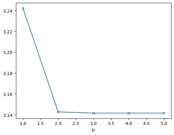
18.3. Poincaré inequality

We are looking for the few lowest critical points / eigenvalues of

\[ \frac{\| \nabla u \|_{L_2}^2}{ \| u \|_{L_2}^2} \]

The smallest eigenvalue \(\lambda_1\) is 0, with the eigenspace being the constant functions. The second-smallest eigenvalue \(\lambda_2\) is the minimum of the Rayleigh quotient, taken the at the \(L_2\)-orthogonal complement to the first eigen-space, i.e. the constants. Thus we get

\[ \| u \|_{L_2}^2 \leq \lambda_2 \, \| \nabla u \|_{L_2}^2 \qquad \forall \, u \in H^1, \; (u,1)_{L_2} = 0 \]

def SetupPoincareProblem(h,p):
    mesh = Mesh(unit_square.GenerateMesh(maxh=h))
    fes = H1(mesh, order=p)
    u,v = fes.TnT()
    H1SemiNorm = BilinearForm(grad(u)*grad(v)*dx).Assemble().mat
    L2Norm = BilinearForm(u*v*dx).Assemble().mat
    pre = Projector(fes.FreeDofs(), range=True)
    return H1SemiNorm, L2Norm, pre, fes

lams = []
for p in range(1,6):
    A,B,P,fes = SetupPoincareProblem(0.3, p)
    evals,evecs = solvers.LOBPCG(A, B, pre=P, num=5, maxit=200, printrates=False, largest=False)
    lams.append([p,sqrt(evals[1])])

print (lams)
plt.xlabel("p")
plt.plot(*zip(*lams), '-x');

[[1, 3.2435260263769448], [2, 3.1427436944464753], [3, 3.141601546084023], [4, 3.1415927925658518], [5, 3.1415940039476355]]

18.4. Korn’s inequality

The symmetrized gradient differential operator on \([H^1(\Omega)]^d\)

\[ \varepsilon(u) := \tfrac{1}{2} \big( \nabla u + (\nabla u)^T \big) \]

plays an important role in solid mechanics. Korn’s first inequality states that, together with an \(L_2\)-norm, it provides an equivalent norm:

\[ \| u \|_{L_2}^2 + \| \varepsilon(u) \|_{L_2}^2 \simeq \| u \|_{H^1}^2 \qquad \forall \, u \in [H^1(\Omega)]^d \]

From Tartar’s theorem follows that the kernel of \(\varepsilon(.)\) is finite dimensional. If the kernel is blocked by essential boundary conditions, the semi-norm becomes a norm.

However, the norm equivalence may depend on the shape of the domain. We perform experiments on the rectangle \((0,L) \times (0,1)\), with Dirichlet boundary conditions at the left side.

def SetupKorn(h,p,L):
    shape = Rectangle(L,1).Face()
    shape.edges.Min(X).name="left"
    mesh = Mesh(OCCGeometry(shape,dim=2).GenerateMesh(maxh=h))
    fes = VectorH1(mesh, order=p, dirichlet="left")
    u,v = fes.TnT()
    EpsSemiNorm = BilinearForm(InnerProduct(Sym(Grad(u)),Sym(Grad(v)))*dx).Assemble().mat
    H1SemiNorm = BilinearForm(InnerProduct(Grad(u),Grad(v))*dx).Assemble().mat
    pre = H1SemiNorm.Inverse(freedofs=fes.FreeDofs(), inverse="sparsecholesky")
    return EpsSemiNorm, H1SemiNorm, pre, fes    

A,B,P,fes = SetupKorn(0.3,3,5)
evals,evecs = solvers.LOBPCG(A, B, pre=P, num=5, maxit=200, printrates=False)
print (evals[0])
gfu = GridFunction(fes)
gfu.vec.data = evecs[0]
Draw (gfu, deformation=True);

0.00406449190545115