52. Modeling Elasticity

Elasticity models the deformation of solid bodies under external forces. We give a short introduction into the modeling of equations.

References are:

• Dietrich Braess: Finite Elements: Theory, Fast Solvers, and Applications in Solid Mechanics, Cambridge University Press, 1997

• Philippe G. Ciarlet: Mathematical Elasticity Vol I, North-Holland, 1988

• Jerrold E. Marsden and Thomas J.R. Hughes.: Mathematical Foundations of Elasticity, Dover, 1983

52.1. Kinematics

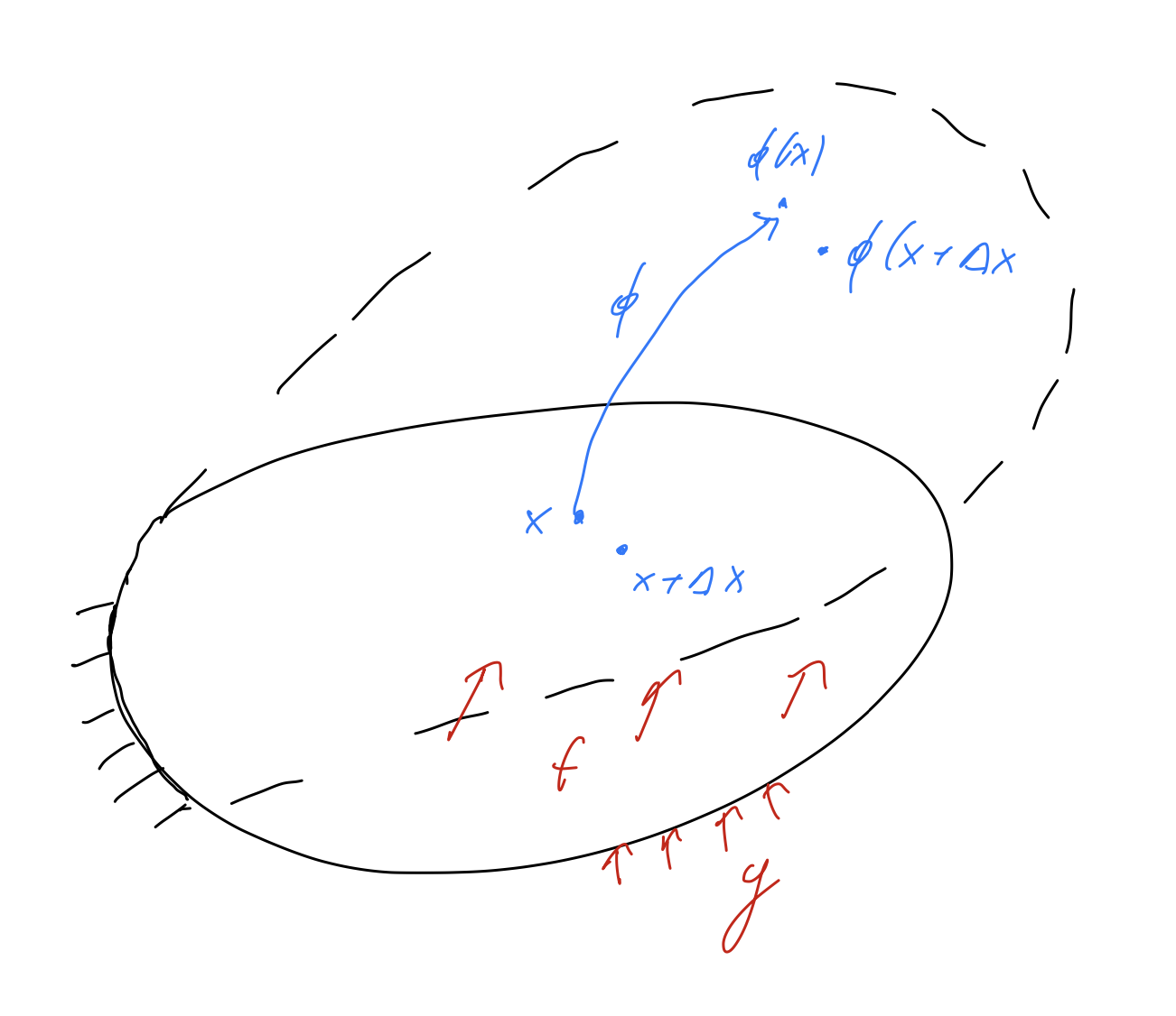
A body in rest is defined by the open set \(\Omega \subset {\mathbb R}^3\). Due to external forces the body is deformed. The so called deformation is a function

\[ \phi : \Omega \rightarrow {\mathbb R}^3. \]

It gives the position of the material point \(x \in \Omega\) of the reference configuration after deformation.

The difference is called displacement:

\[ u(x) = \phi(x) - x \]

Typically, a body is deformed only a little, thus \(\phi \approx id\) and \(u\) is small.

An important quantity is the deformation gradient

\[ F = \nabla \phi \]

A deformation is called feasible if \(\det F > 0\), i.e. the orientation is preserved.

The strength of a deformation is measured by the ration of distances. By squaring the distance the expressions become simpler:

Let \(x\) and \(x + \Delta x\) be two points in the body \(\Omega\). Then there holds for smooth \(\phi\):

\[ \frac{\| \phi(x+\Delta x) - \phi(x)\|^2}{\| x + \Delta x - x \|^2} = \frac{\| F(x) \Delta x + O(\| \Delta x \|^2) \|^2} {\| \Delta x \|^2} = \frac{ \Delta x^T F^T F \Delta x} { \| \Delta x\|^2 } + O(\|\Delta x \|) \]

The relative squared change of length in the point \(x\) into the direction \(\Delta x\) is measured by the so called Cauchy-Green strain tensor

\[ C = F^T F \]

If \(C=I\), the body is not deformed, then \(\phi\) is called a rigid body deformation. One can prove that than \(\phi\) is of the structure

\[ \phi(x) = a + Q x \]

where \(a \in {\mathbb R}^3\) describes the translation, and \(Q\) is a rotation matrix.

The deviation from the rigid body is called Greens’ deformation tensor

\[ E = \frac{1}{2} (C - I) \]

In terms of the deformation one obtains:

\[ E = \frac{1}{2} \big( \nabla u + \nabla u^T + \nabla u^T \nabla u \big). \]

52.2. Elastic material laws

To deform a body, one has to apply work. This is stored as deformation energy in the body. A body is called elastic, if the work is returned after removing the external force.

A constitutive relation is called hyperelastic, if the deformation energy can be point-wise expressed by the Cauchy-Green strain tensor, i.e.:

\[ E_{def} = \int_\Omega W(C(u)) \, dx \]

The energy density \(W\) may depend on the position, i.e. \(W(x, C(u))\), for example if the body consists of different materials.

A constitutive equation is called isotropic, when the material properties are the same in all direction (a counter-example is wood). In an isotropic material the deformation energy stays the same, if the body is rotated (by the rotation \(Q\)) before deformation, i.e.

\[ W (C) = W (F^T F) = W (Q^T F^T F Q) = W(Q^T C Q) \]

Thus, \(W\) is a function of the (real and positive) eigenvalues of \(E\), or also of the coefficients of the characteristic polynomial

\[ \det (\lambda I - E) = \lambda^3 - I_1(E) \lambda^2 + I_2(E) \lambda - I_3(E), \]

called invariants \(I_1(E)\), \(I_2(E)\) and \(I_3(E)\):

\[\begin{align*} I_1(E) & = \operatorname{tr} (E) = \lambda_1 + \lambda_2 + \lambda_3 \\ I_2(E) & = \frac{1}{2} [ (\operatorname{tr} E)^2 - \operatorname{tr} (E^2) ] = \lambda_1 \lambda_2 + \lambda_1 \lambda_3 + \lambda_2 \lambda_3 \\ I_3(E) & = \det (E) = \lambda_1 \lambda_2 \lambda_3 \end{align*}\]

The Rivlin-Ericksen-Theorem says that for isotropic materials there holds

\[ W(E) = W( \operatorname{tr} (E), \operatorname{tr}(E^2), \det (E) ). \]

Let us further assume that \(W(E=0) = 0\) is a local minimum. If \(W\) is smooth, we can apply Taylor exansion:

\[ W(E) = \frac{1}{2} W_{,11} \operatorname{tr} (E)^2 + W_{,2} \operatorname{tr} (E^2) + O(\| E \|^3) \]

Dropping terms of higher order, and calling \(\lambda := W_{,11}\) and \(\mu := W_{,2}\) so we obtain the second order energy density (called Hooke’s law)

\[ W(E) = \frac{\lambda}{2} \operatorname{tr} (E)^2 + \mu E:E, \]

with the notation \(A : B \, := \sum_{ij} A_{ij} B_{ij} = \operatorname{tr} (A : B^T)\). It is similar to an elastic spring: The stored energy is \(\frac{1}{2} k E^2\), with the spring constant \(k\) and elongation \(E\).

52.3. Variational formulation, equilibrium

Let \(V\) be a function space of feasible displacements. On \(\Gamma_D\) the displacement is prescribed (i.e. homogeneous or inhomogeneous Dirichlet boundary conditions).

The total energy consists of the deformation energy, and potential energy due to the external forces:

\[ J(u) = \int_\Omega W(C(u)) \, dx - \int_\Omega f \cdot u \, dx - \int_{\Gamma_N} g \cdot u \, ds \]

Here, \(f\) is a volume force density (e.g. gravity), and \(g\) is a force density on the boundary, called traction. Note that the arguments of \(f\) and \(g\) are the position \(x\) in the reference configuration.

We search for the displacement \(u\) such that the energy is minimal:

\[ \min_{u \in V} J(u) \]

We compute the directional derivative in the direction \(v\) (such that \(u+\varepsilon v\) is feasible as well):

\[ \left< J^\prime(u), v\right> = \int_\Omega \frac{d W}{d C}(C(u)) \frac{d C}{d u}(u) v \, dx - \int_\Omega f v - \int_{\Gamma_N} gv \]

We define the \(2^{nd}\) Piola Kirchhoff stress tensor as

\[ \Sigma = 2 \frac{dW}{dC}. \]

Thus, \(\Sigma\) is a symmetric matrix. From \(C = (I + \nabla u)^T (I + \nabla u)\) there follows

\[ \frac{d C}{d u} v = (I + \nabla u)^T \nabla v + \nabla v^T (I + \nabla u), \]

and thus:

\[\begin{align*} \left< J^\prime(u), v\right> & = \int_\Omega \Sigma : F^T \nabla v - \int_\Omega f v - \int_{\Gamma_N} g v \\ & = \int_\Omega F \Sigma : \nabla v - \int_\Omega f v - \int_{\Gamma_N} g v \end{align*}\]

This term must vanish for all feasible directions \(v\):

\[ \int_\Omega F \Sigma : \nabla v = \int_\Omega f v - \int_{\Gamma_N} g v \qquad \forall \, v \in V(\Omega) \]

From integration by parts we obtain the equilibrium of forces:

\[\begin{align*} -\operatorname{div} F \Sigma & = f \qquad \text{ in } \Omega \\ F \Sigma n & = g \qquad \text{ on } \Gamma_N \end{align*}\]

The matrix $\( P = F \Sigma \)\( is called *\)1^{st}\( Piola-Kirchhoff stress tensor*. In general, \)P$ is not symmetric.

Now we transform integrals to \(\phi(\Omega)\), the deformed body, and set \(v = \tilde v \circ \phi\) with a test-function \(\tilde v\) from a proper space \(V (\phi(\Omega))\). From the chain-rule there follows \(\nabla v = \nabla \tilde v \, F\). Notation: \(J = \det F\):

\[ \int_{\phi(\Omega)} J^{-1} F \Sigma : \nabla \tilde v F \, dx = \int_{\phi(\Omega)} J^{-1} f \tilde v + \int_{\phi(\Gamma_N)} \tilde g \tilde v \qquad \forall \tilde v \in V(\phi(\Omega)) \]

\[ \int_{\phi(\Omega)} J^{-1} F \Sigma F^T : \nabla \tilde v \, dx = \int_{\phi(\Omega)} J^{-1} f \tilde v + \int_{\phi(\Gamma_N)} \tilde g \tilde v \qquad \forall \tilde v \in V(\phi(\Omega)) \]

One obtains \(\tilde g = \frac{ds}{\tilde{ds}} g\) from the transformation of surface measures.

One calls

\[ \sigma := J^{-1} F \Sigma F^T \]

the Cauchy stress tensor. It is symmetric, and satisfies equilibrium of forces on the deformed configuration:

\[\begin{align*} -\operatorname{div} \sigma & = J^{-1} f \qquad \text{ in } \phi(\Omega) \\ \sigma n & = \tilde g \quad \quad \qquad \text{on } \phi(\Gamma_N) \end{align*}\]

Usually, modeling starts with the axiomatic introduction of the Cauchy stress tensor.

52.4. Summary

Summarizing the equation we obtain the non-linear system of partial differential equations of elasticity:

Find the displacement \(u : \Omega \rightarrow {\mathbb R}^3\) such that

• \(F = I + \nabla u\)

• \(C = F^T F, \; \Sigma = 2 \frac{d W}{d C}, \; P = F \Sigma\)

• \(\operatorname{div} P = -f\)

with boundary conditions:

• \(u = u_D\) on \(\Gamma_D\),

• \(P n = g\) on \(\Gamma_N\).

Concerning existence and uniqueness analysis, there are two approaches available:

• The theory by John Ball is based on the minimization of the hyperelastic energy functional. It uses so called poly-convexity. It can prove existence of a solution, but one does not obtain continuous dependency of the solution from data

• The theory by Ciarlet is based on the implicit function theorem. It proves an unique solution depending continuously on data. However, one needs a sufficiently small solution, and high regularity of the problem.