Trace theorems and their applications

15. Trace theorems and their applications#

We consider boundary values of functions in Sobolev spaces. Clearly, this is not well defined for $H^0 = L_2$. But, as we will see, in $H^1$ and higher order Sobolev spaces, it makes sense to talk about $u |_{\partial \Omega}$. The definition of traces is essential to formulate boundary conditions of PDEs in weak form.

We start in one dimension. Let $u \in C^1 ([0,h])$ with some $h > 0$. We multiply $u$ with the cut-off function $1-x/h$ (which does not change the value at $x=0$, and apply the fundamental theorem of calculus:

\[ u(0) = \left(1 - \frac{x}{h} \right) u(x) |_{x=0} = - \int_0^h \left\{ \left(1-\frac{x}{h} \right) u(x) \right\}^\prime \, dx \]

Using the product rule and the Cauchy-Schwarz inequality for $L_2$, we can bound

\[\begin{align*} u(0) & = -\int_0^h \frac{-1}{h} u(x) + \left(1-\frac{x}{h} \right) u^\prime(x) \, dx \\ & \leq \left\| \frac{1}{h} \right\|_{L_2} \| u \|_{L_2} + \left\| 1-\frac{x}{h} \right\|_{L_2} \| u^\prime \|_{L_2} \\ & \simeq h^{-1/2} \| u \|_{L_2(0,h)} + h^{1/2} \| u^\prime \|_{L_2(0,h)}. \end{align*}\]

This estimate includes the scaling with the interval length $h$. If we are not interested in the scaling, we apply Cauchy-Schwarz in ${\mathbb R}^2$, and combine the $L_2$ norm and the $H^1$ semi-norm $\|u^\prime\|_{L_2}$ to the full $H^1$ norm and obtain

\[ |u(0)| \leq \sqrt{h^{-1/2} + h^{1/2} } \sqrt{ \| u \|_{L_2}^2 + \| u^\prime \|_{L_2}^2 } = c \, \| u \|_{H^1}. \]

Next, we extend the trace operator to the whole Sobolev space $H^1$:

Trace theorem in 1D: There is a well defined and continuous trace operator

\[ \operatorname{tr} : H^1((0,h)) \rightarrow {\mathbb R} \]

whose restriction to $C^1([0,h])$ coincides with

\[ u \rightarrow u(0). \]

Proof: Use that $C^1([0,h])$ is dense in $H^1(0,h)$. Take a sequence $u_j$ in $C^1([0,h])$ converging to $u$ in $H^1$-norm. This sequence is Cauchy. By continuity of the boundary trace, the sequence of boundary values $u_j(0)$ is Cauchy as well, and thus converges to a limit $u_0$. The limit is independent of the choice of the sequence $u_j$. This allows to define $\operatorname{tr} u := u_0$. $\Box$

Now, we extend this 1D result to domains in more dimensions. Let $\Omega$ be bounded, $\partial \Omega$ be Lipschitz, and consists of $M$ pieces $\Gamma_i$ of smoothness $C^1$.

We can construct the following covering of a neighbourhood of $\partial \Omega$ in $\Omega$: Let $Q = (0,1)^2$. For $1 \leq i \leq M$, let $s_i \in C^1 (Q, \Omega)$ be invertible and such that $\left\| s_i^\prime \right\|_{L_\infty} \leq c$, $\| (s_i^\prime)^{-1} \|_{L_\infty} \leq c$, and $\operatorname{det} s_i^\prime > 0$. The domains $S_i := s_i(Q)$ are such that $s_i( (0,1) \times \{ 0 \} ) = \Gamma_i$, and the parameterizations match on $s_i( \{ 0,1 \} \times (0,1) )$.

Trace Theorem: There exists a well defined and continuous operator

\[ \operatorname{tr} : H^1 (\Omega) \rightarrow L_2(\partial \Omega) \]

which coincides with $u|_{\partial \Omega}$ for $u \in C^1(\overline{\Omega})$.

Proof: Again, we prove that

\[ \operatorname{tr} : C^1(\overline{\Omega}) \rightarrow L_2(\partial \Omega) : u \rightarrow u |_{\partial \Omega} \]

is a bounded operator w.r.t. the norms $\|.\|_{H^1(\Omega)}$ and $\|.\|_{L_2(\partial \Omega)}$, and conclude by density.

We start proving the trace estimate on the square $Q := (0,1)^2$, and taking boundary values on the bottom side $\Gamma_b := (0,1) \times \{0\}$. For every $\xi \in (0,1)$ we apply the one-dimensional trace inequality in $y$-direction:

\[ | u(\xi, 0)|^2 \leq c \int_0^1 \left\{ u(\xi,\eta)^2 + \left(\frac{\partial u}{\partial \eta}(\xi,\eta)\right)^2 \right\} \, d \eta \qquad \forall \, \xi \in (0,1) \]

The result follows from integrating over $\xi$ and Fubini:

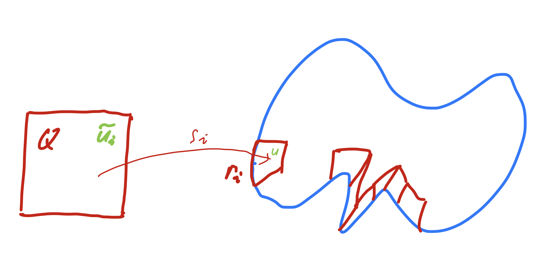
\[\begin{align*} \| u \|_{L_2(\Gamma_b)}^2 &= \int_0^1 | u(\xi, 0)|^2 \, d\xi \\ & \leq c \, \int_0^1 \int_0^1 \left\{ u(\xi,\eta)^2 + \left(\frac{\partial u}{\partial \eta}(\xi,\eta) \right)^2 \right\} \, d \eta \, d \xi \\ & \leq c \, \| u \|_{H^1(Q)}^2. \end{align*}\]

We use the partitioning of $\partial \Omega$ into non-overlapping parts $\Gamma_i$, $1 \leq i \leq M$. For each part $\Gamma_i$ we define an injective transformation $s_i : \overline Q \rightarrow \overline \Omega$ such that the bottom edge of $Q$ is mapped onto $\Gamma_i$. We define $S_i = s_i(Q)$. We assume that $s_i^\prime$ and $(s_i^\prime)^{-1}$ are bounded functions a.e.

This allows to pull-back functions $u \in H^1(S_i)$ locally to the square domain $Q$:

\[ \tilde u_i = u \circ s_i \]

We transfer the $L_2(\Gamma_i)$-norms to the bottom edges:

\[\begin{align*} \| \operatorname{tr} u \|_{L_2(\partial \Omega)}^2 & = % \sum_{i=1}^M \| u \|_{L_2(\Gamma_i)}^2 = \sum_{i=1}^M \int_{\Gamma_i} u(x)^2 \, dx \\ & = \sum_{i=1}^M \int_0^1 u(s_i(\xi,0))^2 \left| \frac{\partial s_i}{\partial \xi} (\xi, 0) \right| \, d \xi \\ & \leq c \sum_{i=1}^M \int_0^1 \tilde u_i(\xi,0)^2 \, d \xi \end{align*}\]

To transform the $H^1$-norm, we use the chain-rule

\[ \tilde u_i^\prime = (u^\prime \circ s_i) \; s_i^\prime \]

Since $s_i^\prime$ and $(s_i^\prime)^{-1}$ are uniformly bounded, we get

\[ | \nabla \tilde u_i (x) | \simeq | \nabla u (s_i(x) | \quad \forall \, a.e. \, x \in Q, \]

and, furthermore

\[ \| \nabla \tilde u_i \|_{L_2(Q)} \simeq \| \nabla u \|_{L_2(S_i)} \]

Combining the estimates we have proven

\[\begin{align*} \| \operatorname{tr} u \|_{\partial \Omega}^2 & \simeq \sum_i \| \tilde u_i \|_{L_2(\Gamma_b)}^2 \preceq \sum_i \| \tilde u_i \|_{H^1(Q)}^2 \\ & \simeq \sum_i \| u \|_{H^1(S_i)}^2 \preceq \| u \|_{H^1(\Omega)}^2 \end{align*}\]

$\Box$

Considering the trace operator from $H^1(\Omega)$ to $L_2(\partial \Omega)$ is not sharp with respect to the norms. We will improve the embedding later.

By means of the trace operator we define the sub-space

\[ H_0^1(\Omega) = \{ u \in H^1(\Omega) : \operatorname{tr} \, u = 0 \} \]

It is a true sub-space, since $u = 1$ does belong to $H^1$, but not to $H_0^1$. It is a closed sub-space, since it is the kernel of a continuous operator.

By means of the trace inequality, one verifies that the linear-form

\[ g(v) := \int_{\Gamma_N} g \, \operatorname{tr} \, v \, dx \]

is bounded on $H^1$.

Using the Cauchy-Schwarz inequality on $L_2(\Gamma_N)$, and continuity of the trace operator we obtain:

\[\begin{align*} | g(v) | \leq & \| g \|_{L_2(\Gamma_N)} \| \operatorname{tr} v \|_{L_2(\Gamma_N)} \\ \leq & \| g \|_{L_2(\Gamma_N)} \| \operatorname{tr} \|_{H^1(\Omega)\rightarrow L_2(\Gamma_N)} \| v \|_{H^1(\Omega)} \end{align*}\]

Thus, the dual-norm of the linear-form is bounded by

\[ \| g(\cdot) \|_{H^1(\Omega)^*} = \| g \|_{L_2} \| \operatorname{tr} \| \]

15.1. Integration by parts#

The definition of the trace allows us to perform integration by parts in $H^1$:

\[ \int_{\Omega} \nabla u \varphi \, dx = -\int_\Omega u \operatorname{div} \, \varphi \, dx + \int_{\partial \Omega} \operatorname{tr} u \, \varphi \cdot n \, dx \qquad \forall \, \varphi \in [C^1(\overline{\Omega})]^2 \]

The definition of the weak derivative (e.g. the weak gradient) looks similar. However, it allows only test functions $\varphi$ with compact support in $\Omega$, i.e., having zero boundary values. Only by choosing a normed space, for which the trace operator is well defined, we can state and prove integration by parts. Again, the short proof is based on the density of $C^1(\overline \Omega)$ in $H^1$.

15.2. Sobolev spaces over sub-domains#

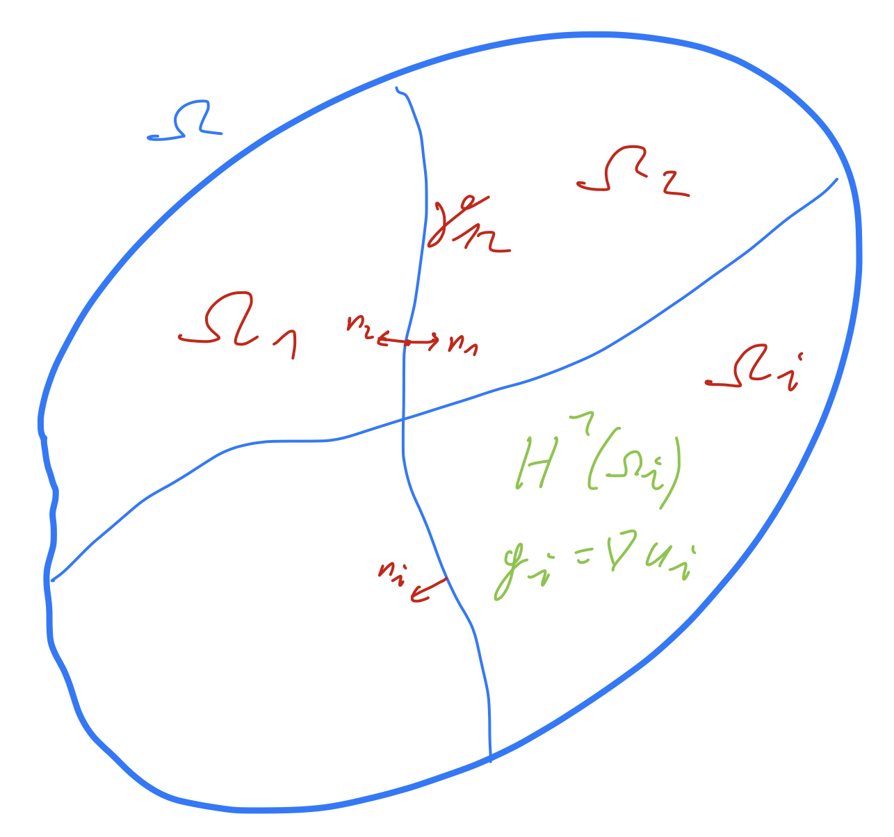
Let $\Omega$ consist of $M$ Lipschitz-continuous sub-domains $\Omega_i$ such that

$\overline \Omega = \cup_{i=1}^M \overline \Omega_i$
$\Omega_i \cap \Omega_j = \emptyset \quad \mbox{ if } i \neq j$

The interfaces are $\gamma_{ij} = \overline \Omega_i \cap \overline \Omega_j$. The outer normal vector of $\Omega_i$ is $n_i$.

Theorem: Let $u \in L_2(\Omega)$ such that

$u_i := u|_{\Omega_i}$ is in $H^1(\Omega_i)$, and $g_i = \nabla u_i$ is its weak gradient

the traces on common interfaces coincide:

\[ \operatorname{tr}_{\gamma_{ij}} u_i = \operatorname{tr}_{\gamma_{ij}} u_j \]

Then $u$ belongs to $H^1(\Omega)$. Its weak gradient $g = \nabla u$ fulfills $g|_{\Omega_i} = g_i$.

Proof: We have to verify that $g \in L_2(\Omega)^d$, defined by $g |_{\Omega_i} = g_i$, is the weak gradient of $u$, i.e.,

\[ \int_\Omega g \cdot \varphi \, dx = - \int_\Omega u \, \operatorname{div} \varphi \, dx \qquad \forall \, \varphi \in [C_0^\infty(\Omega)]^d \]

We split the integral over sub-domains, use the definition of the local gradient, perform integration by parts on the sub-domains, and combine boundary terms from $\Omega_i$ and $\Omega_j$ to the common interface $\gamma_{ij}$:

\[\begin{align*} \int_\Omega g \cdot \varphi \, dx & = \sum_{i=1}^M \int_{\Omega_i} g_i \cdot \varphi \, dx = \sum_{i=1}^M \int_{\Omega_i} \nabla u_i \cdot \varphi \, dx \\ & = \sum_{i=1}^M -\int_{\Omega_i} u_i \operatorname{div} \varphi \, dx + \int_{\partial \Omega_i} \operatorname{tr} u_i \, \varphi \cdot n_i \, ds \\ & = -\int_\Omega u \operatorname{div} \varphi \, dx + \sum_{\gamma_{ij}} \int_{\gamma_{ij}} \left\{ \operatorname{tr}_{\gamma_{ij}} u_i \, \varphi \cdot n_i + \operatorname{tr}_{\gamma_{ij}} u_j \, \varphi \cdot n_j \right\} \, ds \\ & = -\int_\Omega u \, \operatorname{div} \varphi \, dx \end{align*}\]

We have used that $\varphi = 0$ on $\partial \Omega$, and $n_i = -n_j$ on $\gamma_{ij}$. $\Box$

Applications of this theorem are (conforming nodal) finite element spaces. The partitioning $\Omega_i$ is the mesh. On each sub-domain, i.e., on each element $T$, the functions are polynomials and thus in $H^1(T)$. The finite element functions are constructed to be continuous, i.e., the traces match on the interfaces. Thus, the finite element space is a sub-space of $H^1$.

15.3. Extension operators#

Some estimates are elementary to verify on simple domains such as squares $Q$. One technique to transfer these results to general domains is to extend a function $u \in H^1(\Omega)$ onto a larger square $Q$, apply the result for the square, and restrict the result onto the general domain $\Omega$. This is now the motivation to study extension operators.

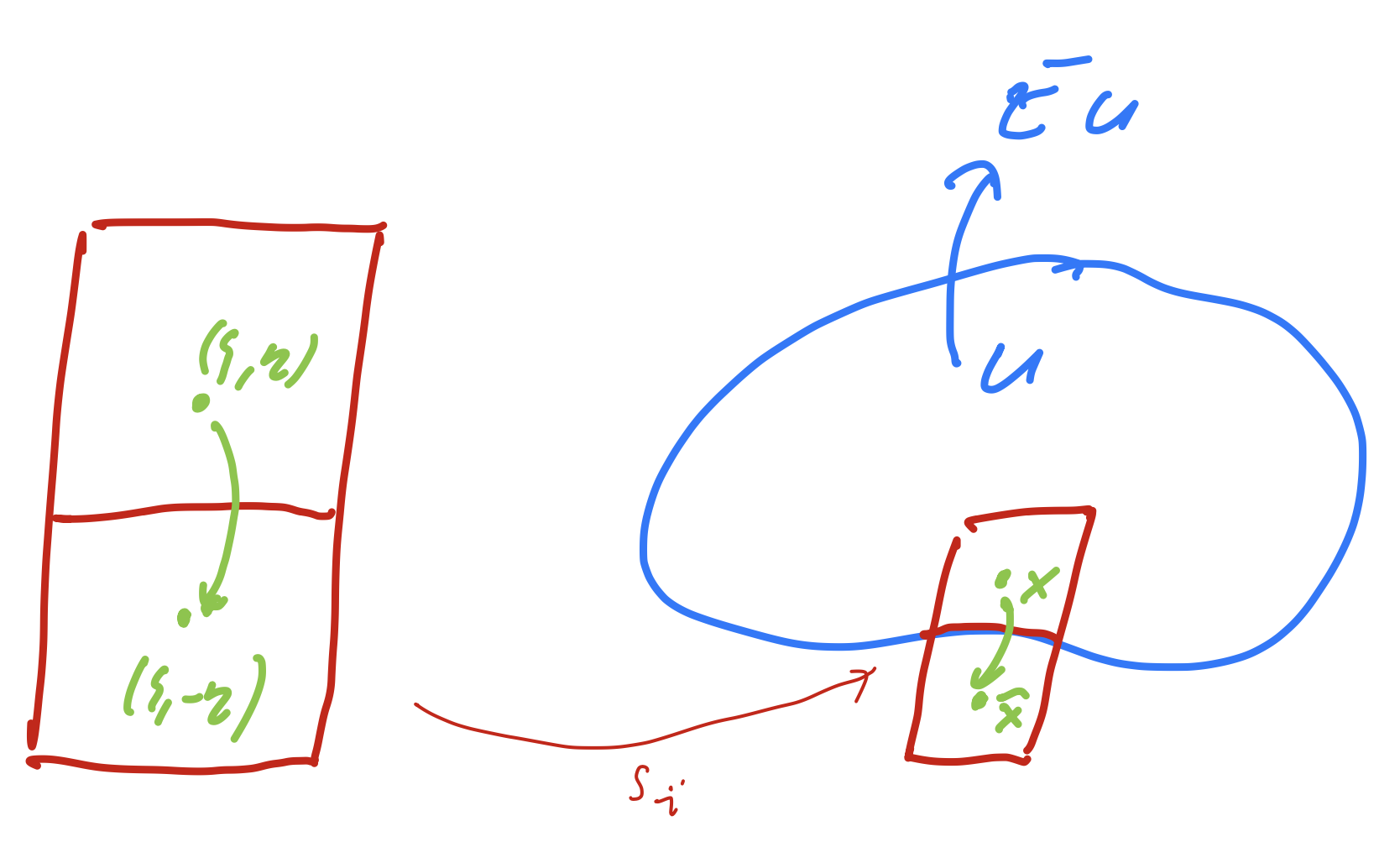
We construct a non-overlapping covering $\{ S_i \}$ of a neighbourhood of $\partial \Omega$ on both sides. Let $\partial \Omega = \cup \Gamma_i$ consist of smooth parts. Let $s : (0,1) \times (-1,1) \rightarrow S_i : (\xi, \eta) \rightarrow x$ be an invertible function such that

\[\begin{eqnarray*} s_i ( (0,1) \times (0,1) ) & = & S_i \cap \Omega \\ s_i ( (0,1) \times \{ 0 \} ) & = & \Gamma_i \\ s_i ( (0,1) \times (-1,0) ) & = & S_i \setminus \overline \Omega \end{eqnarray*}\]

Assume that $\| \frac{ds_i}{dx} \|_{L_\infty}$ and $\| \left( \frac{ds_i}{dx} \right)^{-1} \|_{L_\infty}$ are bounded.

This defines an invertible mapping $x \rightarrow \hat x (x)$ from the inside to the outside by

\[ \hat x(x) = s_i (\xi(x), -\eta(x)). \]

The mapping preserve the boundary $\Gamma_i$. The transformations $s_i$ should be such that $x \rightarrow \hat x$ is consistent at the interfaces between $S_i$ and $S_j$.

With the flipping operator $f : (\xi, \eta) \rightarrow (\xi, -\eta)$, the mapping is the composite $\hat x(x) = s_i (f(s_i^{-1}))$. From that, we obtain the bound

\[ \left\| \frac{d \hat x}{d x } \right\| \leq \left\| \frac{ds}{dx} \right\| \left\| \left( \frac{ds}{dx} \right)^{-1} \right\|. \]

Define the domain $\widetilde \Omega = \Omega \cup S_1 \cup \ldots \cup S_M$.

We define the extension operator by

(15.1)#\[\begin{equation} \begin{array}{rcll} (E u) (\hat x) & = & u(x) & \qquad \forall \, x \in \cup S_i \\ (Eu) (x) & = & u(x) & \qquad \forall \, x \in \Omega \end{array} \end{equation}\]

Theorem: The extension operator $E : H^1(\Omega) \rightarrow H^1(\widetilde \Omega)$ is well defined and bounded with respect to the norms

\[ \| E u \|_{L_2(\widetilde \Omega)} \leq c \, \| u \|_{L_2(\Omega)} \]

and

\[ \| \nabla E u \|_{L_2(\widetilde \Omega)} \leq c \, \| \nabla u \|_{L_2(\Omega)} \]

Proof: Let $u \in C^1(\overline \Omega)$. First, we prove the estimates for the individual pieces $S_i$:

\[ \int_{S_i \setminus \Omega} E u (\hat x)^2 \, d \hat x = \int_{S_i \cap \Omega} u (x)^2 \, \det \left( \frac{d \hat x}{d x} \right) d x \leq c \| u \|_{L_2(S_i \cap \Omega)}^2 \]

For the derivatives we use

\[ \frac{d E u(\hat x)}{d\hat x} = \frac{d u(x(\hat x))}{d \hat x} = \frac{d u}{dx} \frac{dx}{d \hat x}. \]

Since $\frac{d x}{d \hat x}$ and $(\frac{d x}{d \hat x})^{-1} = \frac{d \hat x}{dx}$ are bounded, one obtains

\[ | \nabla_{\hat x} E u (\hat x) | \simeq | \nabla_x u(x) |, \]

and

\[ \int_{S_i \setminus \Omega} | \nabla_{\hat x} E u |^2 \, d \hat x \leq c \int_{S_i \cap \Omega} | \nabla u |^2 \, dx \]

These estimates prove that $E$ is a bounded operator into $H^1$ on the sub-domains $S_i \setminus \Omega$. The construction was such that for $u \in C^1(\overline \Omega)$, the extension $E u$ is continuous across $\partial \Omega$, and also across the individual $S_i$. By Theorem~\ref{theo_subdomainh1}, $E u $ belongs to $H^1 (\widetilde \Omega)$, and

\[ \| \nabla E u \|_{L_2(\widetilde \Omega)}^2 = \| \nabla u \|_{\Omega}^2 + \sum_{i=1}^M \| \nabla u \|_{S_i \setminus \Omega}^2 \leq c \| \nabla u \|_{L_2(\Omega)}^2, \]

By density, we get the result for $H^1(\Omega)$. Let $u_j \in C^1(\overline \Omega) \rightarrow u$, than $u_j$ is Cauchy, $E u_j$ is Cauchy in $H^1(\widetilde \Omega)$, and thus converges to $u \in H^1(\widetilde \Omega)$.

The extension of functions from $H_0^1(\Omega)$ onto larger domains is trivial: Extension by $0$ is a bounded operator. One can extend functions from $H^1(\Omega)$ into $H_0^1(\widetilde \Omega)$, and further, to an arbitrary domain by extension by $0$.

For $\hat x = s_i(\xi, -\eta)$, $\xi, \eta \in (0,1)^2$, define the extension $$ E_0 u (\hat x) = (1-\eta) \, u(x) $$ This extension vanishes at $\partial \widetilde \Omega$

Theorem: The extension $E_0$ is an extension from $H^1(\Omega)$ to $H_0^1(\widetilde \Omega)$. It is bounded w.r.t.

\[ \| E_0 u \|_{H^1(\widetilde \Omega)} \leq c \| u \|_{H^1(\Omega)} \]

Proof: Exercises

In this case, it is not possible to bound the gradient term only by gradients. To see this, take the constant function on $\Omega$. The gradient vanishes, but the extension is not constant.

15.4. The trace space $H^{1/2}$#

The trace operator is continuous from $H^1(\Omega)$ into $L_2(\partial \Omega)$. But, not every $g \in L_2(\partial \Omega)$ is a trace of some $u \in H^1(\Omega)$. We will motivate why the trace space is the fractional order Sobolev space $H^{1/2}(\partial \Omega)$.

We introduce a space with a stronger norm, such that the trace operator is still continuous, and also surjective. Let $V = H^1(\Omega)$, and define the trace space as the range of the trace operator

\[ W = \{ \operatorname{tr} \, u : u \in H^1(\Omega) \} \]

with the norm

\[ \| \operatorname{tr} u \|_W = \inf_{v \in V \atop \operatorname{tr} \, u = \operatorname{tr} \, v } \| v \|_V. \]

This is indeed a norm on $W$. The trace operator is continuous from $V \rightarrow W$ with norm $1$.

Lemma: The space $(W, \|.\|_W)$ is a Banach space. For all $g \in W$ there exists an $u \in V$ such that $\operatorname{tr} \, u = g$ and $\| u \|_V = \| g \|_W$

Proof: The kernel space $V_0 := \{ v : \operatorname{tr} \, v = 0 \}$ is a closed sub-space of $V$. If $\operatorname{tr} \, u = \operatorname{tr} \, v$, then $z := u - v \in V_0$. We can rewrite

\[ \| \operatorname{tr} \, u \|_W = \inf_{z \in V_0} \| u - z \|_V = \| u - P_{V_0} u \|_V \qquad \forall \, u \in V \]

Now, let $g_n = \operatorname{tr} \, u_n \in W$ be a Cauchy sequence. This does not imply that $u_n$ is Cauchy, but $P_{V_0^\bot} u_n$ is Cauchy in $V$:

\[ \| P_{V_0^\bot} (u_n - u_m) \|_V = \| \operatorname{tr} \, (u_n - u_m) \|_W. \]

The $P_{V_0^\bot} u_n$ converge to some $u \in V_0^\bot$, and $g_n$ converge to $g := \operatorname{tr} \, u$. $\Box$

The minimizer fulfills

\[ \operatorname{tr} \, u = g \qquad \mbox{and} \qquad (u,v)_V = 0 \qquad \forall \, v \in V_0. \]

This means that $u$ is the solution of the weak form of the Dirichlet problem

\[\begin{split} \begin{array}{rcll} -\Delta u + u & = & 0 \qquad & \mbox{ in } \Omega \\ u & = & g \qquad & \mbox{ on } \partial \Omega. \end{array} \end{split}\]

To give an explicit characterization of the norm $\|.\|_W$, we introduce Hilbert space interpolation:

15.5. Interpolation spaces#

To explain the idea we expand $u \in L_2(0,1)$ in a Fourier-sine-series

\[ u = \sum_{k=1}^\infty u_k \sin (k\pi x) \]

with Fourier coefficients

\[ u_k = 2 \int_0^1 u(x) \sin (k\pi x) \, dx \]

The $L_2$-norm is (by Parseval’s theorem)

\[ \| u \|_{L_2}^2 = \tfrac{1}{2} \sum_{k=1}^\infty u_k^2. \]

Formally, its derivative is

\[ u^\prime(x) = \sum_{k=1}^\infty u_k k \pi \cos (k \pi x), \]

and the $H^1$ semi-norm (which is here actually equivalent to the norm) is

\[ | u |_{H^1}^2 = \frac{\pi^2}{2} \sum_{k=1}^\infty k^2 u_k^2 \]

The function $u$ lies in $H_0^1 \subset L_2$ if and only if this is a finite sum, i.e. $(k u_k)_{k \in {\mathbb N}}$ lies in $l_2$.

This motivates to define the family of interpolation spaces

\[ H^s_0 = [L_2, H_0^1]_s \qquad \text{for} \; s \in (0,1) \]

of functions

\[ u(x) = \sum_{k=1}^\infty u_k \sin (k \pi x) \qquad \text{such that} \; \sum_{k=1}^\infty k^{2s} u_k^2 < \infty \]

The norms are

\[ \| u \|_{H^s}^2 = \sum_{k=1}^\infty k^{2s} u_k^2 \]

For the limiting values $s=0$ and $s=1$, the interpolation space are $L_2$ and $H_0^1$, respectively.

Since all terms have zero boundary values, the Fourier-sine series spans $H_0^1$. If we use the Fourier-cosine series instead, we obtain the whole space $H^1$.

15.5.1. General definition:#

Let $V_1 \subset V_0$ be two Hilbert spaces, such that $V_1$ is dense in $V_0$, and the embedding operator $id : V_1 \rightarrow V_0$ is compact. We can pose the eigen-value problem: Find $z \in V_1$, $\lambda \in {\mathbb R}$ such that

\[ (z, v)_{V_1} = \lambda (z, v)_{V_0} \qquad \forall \, v \in V_1. \]

There exists a sequence of eigen-pairs $(z_k, \lambda_k)$ such that $\lambda_k \rightarrow \infty$. The $z_k$ form an orthonormal basis in $V_0$, and an orthogonal basis in $V_1$.

The converse is also true. If $z_k$ is a basis for $V_0$, and the eigenvalues $\lambda_k \rightarrow \infty$, then the embedding $V_1 \subset V_0$ is compact.

Given $u \in V_0$, it can be expanded in the orthonormal eigen-vector basis:

\[ u = \sum_{k=0}^\infty u_k z_k \qquad \mbox{with} \qquad u_k = (u, z_k)_{V_0} \]

The $\|.\|_{V_0}$ - norm of $u$ is

\[ \| u \|_{V_0}^2 = (\sum_k u_k z_k, \sum_l u_l z_l)_{V_0} = \sum_{k,l} u_k u_l (z_k,z_l)_{V_0} = \sum_k u_k^2. \]

If $u \in V_1$, then

\[ \| u \|_{V_1}^2 = (\sum_k u_k z_k, \sum_l u_l z_l)_{V_1} = \sum_{k,l} u_k u_l (z_k,z_l)_{V_1} = \sum_{k,l} u_k u_l \lambda_k (z_k,z_l)_{V_0} = \sum_k u_k^2 \lambda_k \]

The sub-space space $V_1$ consists of all $u = \sum u_k z_k$ such that $\sum_k \lambda_k u_k^2$ is finite. This suggests the definition of the interpolation norm

\[ \| u \|_{V_s}^2 = \sum_k (u, z_k)_{V_0}^2 \lambda_k^s, \]

and the interpolation space $V_s = [V_0, V_1]_s$ as

\[ V_s = \{ u \in V_0 : \| u \|_{V_s} < \infty \}. \]

We have been fast with using infinite sums. To make everything precise, one first works with finite dimensional sub-spaces $\{ u : \exists n \in {\mathbb N} \mbox{ and } u = \sum_{k=1}^n u_k z_k \}$, and takes the closure.

In our case, we apply Hilbert space interpolation to $H^1(0,1) \subset L_2(0,1)$. The eigen-value problem is to find $z_k \in H^1$ and $\lambda_k \in {\mathbb R}$ such that

\[ (z_k, v)_{L_2} + (z_k^\prime, v^\prime)_{L_2} = \lambda_k \, (z_k, v)_{L_2} \qquad \forall \, v \in H^1 \]

By definition of the weak derivative, there holds $(z_k^\prime)^\prime = (1-\lambda_k) z_k$, i.e., $z^k \in H^2$. Since $H^2 \subset C^0$, there holds also $z \in C^2$, and a weak solution is also a solution of the strong form

(15.2)#\[\begin{equation} \begin{array}{rcll} z_k - z_k^{\prime \prime} & = & \lambda_k z_k \qquad & \mbox{ on } (0,1) \\ z_k^\prime(0) = z_k^\prime(1) & = & 0 \end{array} \end{equation}\]

All solutions, normalized to $\| z_k \|_{L_2} = 1$, are

\[ z_0 = 1 \qquad \lambda_0 = 1 \]

and, for $k \in {\mathbb N}$,

\[ z_k(x) = \sqrt{2} \cos (k \pi x) \qquad \lambda_k = 1 + k^2 \pi^2. \]

Indeed, expanding $u \in L_2$ in the $\cos$-basis $u = u_0 + \sum_{k=1}^\infty u_k \sqrt2 \cos (k \pi x)$, one has

\[ \| u \|_{L_2}^2 = \sum_{k=0}^\infty (u, z_k)_{L_2}^2 \]

and

\[ \| u \|_{H^1}^2 = \sum_{k=0}^\infty (1+k^2 \pi^2) (u, z_k)_{L_2}^2 \]

Differentiation adds a factor $k \pi$. Hilbert space interpolation allows to define the fractional order Sobolev norm ($s \in (0,1)$)

\[ \| u \|_{H^s(0,1)}^2 = \sum_{k=0}^\infty (1+k^2 \pi^2)^s (u,z_k)_{L_2}^2 \]

15.5.2. The trace space on one edge of the square#

We consider the trace $\operatorname{tr}|_E$ of $H^1((0,1)^2)$ on the bottom edge $E = (0,1) \times \{ 0 \}$. For $g \in W_E := \operatorname{tr}_E H^1((0,1)^2)$, the norm $\| g \|_W$ is defined by

\[ \| g \|_W = \| u_g \|_{H^1}, \]

where $u_g$ solves the Dirichlet problem $u_g|_E = g$, and $(u_g,v)_{H^1} = 0 \; \forall \, v \in H^1$ such that $\operatorname{tr}_E v = 0$.

Since $W \subset L_2(E)$, we can expand $g$ in the $L_2$-orthonormal cosine basis $z_k$

\[ g(x) = \sum_{k=0}^{\infty} g_k z_k(x) \]

The Dirichlet problems for the $z_k$,

\[\begin{split} \begin{array}{rcll} -\Delta u_k + u_k & = & 0 \qquad & \mbox{in } \Omega \\ u_k & = & z_k \qquad & \mbox{on } E \\ \frac{\partial u_k}{\partial n} & = & 0 \qquad & \mbox{on } \partial \Omega \setminus E, \end{array} \end{split}\]

have the explicit solution

\[ u_0(x,y) = 1 \]

and

\[ u_k(x,y) = \sqrt 2 \cos (k \pi x) \frac{e^{k \pi (1-y)} + e^{-k \pi (1-y)}}{e^{k \pi} + e^{-k \pi}}. \]

Ignoring constant factors, there holds

\[ \| u_k \|_{L_2}^2 \simeq (k+1)^{-1} \]

and

\[ \| \nabla u_k \|_{L_2}^2 \simeq k \]

Furthermore, the $u_k$ are orthogonal in $(.,.)_{H^1}$. Thus, $u_g = \sum_k g_k u_k$ has the norm

\[ \| u_g \|_{H^1}^2 = \sum g_k^2 \| u_k \|_{H^1}^2 \simeq \sum_k g_k^2 (1+k). \]

This norm is equivalent to $H^{1/2}(E)$.

We have proven that the trace space onto one edge is the interpolation space $H^{1/2}(E)$. This is also true for general domains (Lipschitz, with piecewise smooth boundary).