73. The Gradient Method

In this section we assume that \(A\) is SPD.

We define the function \(f : {\mathbb R}^n \rightarrow {\mathbb R}\) as

\[ f(x) = \tfrac{1}{2} x^T A x - b^T x. \]

The gradient and Hessian matrix of \(f\) are

\[\begin{align*} \nabla f(x) & = A x - b, \\ \nabla^2 f & = A. \end{align*}\]

Since \(A\) is positive definite, \(f\) is convex and there exists a unique minimizer of

\[ \min_{x \in {\mathbb R}^n} f(x) \]

characterized by \(\nabla f = 0\), i.e. the solution of the linear system \(A x = b\). Thus, the linear system is equivalent to the minimization problem.

There holds

\[ f(x) = f(x^\ast) + \tfrac{1}{2} \| x - x^\ast \|_A^2, \]

which is simply verified by calculation:

\[\begin{align*} f(x^\ast) + \tfrac{1}{2} \| x - x^\ast \|_A^2 & = \tfrac{1}{2} {x^\ast}^T A x^\ast - b^T x^\ast + \tfrac{1}{2}(x - x^\ast)^T A (x - x^\ast) \\ & = {x^\ast}^T A x^\ast - b^T x^\ast + \tfrac{1}{2} x^T A x - x^T A x^\ast \\ & = \tfrac{1}{2} x^T A x - b^T x = f(x) \end{align*}\]

The error in energy norm is directly related to the distance to the minimum.

We apply the gradient method: The next iterate \(x^{k+1}\) is obtained by moving from \(x^k\) into the direction of the negative gradient:

\[\begin{eqnarray*} x^{k+1} & = & x^k - \alpha \nabla f(x^k) \\ & = & x^k + \alpha r \qquad \text{with} \qquad r = b - A x^k \end{eqnarray*}\]

The optimal parameter \(\alpha\) can be obtained by line-search:

\[ \min_{\alpha \in {\mathbb R}} f(x^k + \alpha r) \]

i.e.

\[ \min_\alpha \tfrac{1}{2} (x^k + \alpha r)^T A (x^k + \alpha r) - b^T (x^k + \alpha r) \]

what is a minimization problem of a convex, quadratic function

\[ \min_{\alpha \in {\mathbb R}} \tfrac{1}{2} r^T A r \, \alpha^2 - (b-A x^k)^T r \, \alpha + \tfrac{1}{2} {x^k}^T A x^k - b^T x^k \]

The optimal value \(\alpha_\text{opt}\) is found as

\[ \alpha_\text{opt} = \frac{r^T r}{r^T A r} \]

The gradient method looks like:

Given \(x^0\)
for \(k = 0, 1, 2, \ldots\)
\(\qquad r = b - A x^k\)
\(\qquad \alpha = \frac{r^T r}{r^T A r}\)
\(\qquad x^{k+1} = x^k + \alpha r\)

In this version, one needs two matrix-vector products with \(A\). By updating the residual one can avoid the second product:

Given \(x^0\)
\(r^0 = b - A x^0\)
for \(k = 0, 1, 2, \ldots\)
\(\qquad p = A r^k\)
\(\qquad \alpha = \frac{{r^k}^T r^k}{{r^k}^T p}\)
\(\qquad x^{k+1} = x^k + \alpha r^k\)
\(\qquad r^{k+1} = r^k - \alpha p\)

from ngsolve import *
mesh = Mesh(unit_square.GenerateMesh(maxh=0.1))
fes = H1(mesh, order=1)
u,v = fes.TnT()
a = BilinearForm(grad(u)*grad(v)*dx+10*u*v*dx).Assemble()
f = LinearForm(x*y*v*dx).Assemble()
gfu = GridFunction(fes)

The code in NGSolve:

r = f.vec.CreateVector()
p = f.vec.CreateVector()

gfu.vec[:] = 0
r.data = f.vec
err0 = Norm(r)
its = 0
errhist = []
while True:
    p.data = a.mat * r
    err2 = InnerProduct(r,r)
    alpha = err2 / InnerProduct(r,p)

    # print ("iteration", its, "res=", sqrt(err2))
    errhist.append (sqrt(err2))
    gfu.vec.data += alpha * r
    r.data -= alpha * p
    if sqrt(err2) < 1e-8 * err0 or its > 10000: break
    its = its+1
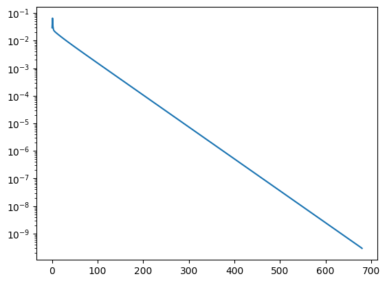
print ("needed", len(errhist), "iterations")

needed 677 iterations

import matplotlib.pyplot as plt
plt.yscale('log')
plt.plot(errhist);

We observe that the gradient method converges similar fast as the Richardson iteration, but without the need of a good chosen relaxation parameter \(\alpha\).

The comparison to Richardson iteration allows also to estimate the error reduction of the gradient method. Let $\( \tilde x^{k+1} = x^k - \alpha_\text{Rich} (b - A x^k) \)$ be one step of Richardson. Then, using the optimality property along the search direction of the gradient method, we observe

\[\begin{align*} \| x^{k+1} - x^\ast \|_A^2 &= 2 \, (f(x^{k+1}) - f(x^\ast)) \leq 2 \, ( f (\tilde x^{k+1}) - f(x^\ast) ) \\ &= \| \tilde x^{k+1} - x^\ast \|_A^2 \leq \rho_{Rich} \| x^k - x^\ast \|_A \end{align*}\]

One step of the gradient method reduces the error (measured in energy norm) at least as much as one step of the Richardson method.