26. A posteriori error estimates

We will derive methods to estimate the error of the computed finite element approximation. Such a posteriori error estimates may use the finite element solution \(u_h\), and input data such as the source term \(f\).

\[ \eta(u_h, f) \]

An error estimator is called reliable, if it is an upper bound for the error, i.e., there exists a constant \(C_1\) such that

\[ \| u - u_h \|_V \leq C_1 \, \eta(u_h, f) \]

An error estimator is efficient, if it is a lower bound for the error, i.e., there exists a constant \(C_2\) such that

\[ \| u - u_h \|_V \geq C_2 \, \eta(u_h, f). \]

The constants may depend on the domain, and the shape of the triangles, but may not depend on the source term \(f\), or the (unknown) solution \(u\).

One use of the a posteriori error estimator is to know the accuracy of the finite element approximation. A second one is to guide the construction of a new mesh to improve the accuracy of a new finite element approximation.

The usual error estimators are defined as sum over element contributions:

\[ \eta^2 (u_h, f) = \sum_{T \in {\cal T}} \eta_T^2 (u_h, f) \]

The local contributions should correspond to the local error. For the common error estimators there hold the local efficiency estimates

\[ \| u - u_h \|_{H^1(\omega_T)} \geq C_2 \, \eta_T(u_h, f). \]

The patch \(\omega_T\) contains \(T\) and all its neighbor elements.

In the following, we consider the Poisson equation \(-\Delta u = f\) with homogeneous Dirichlet boundary conditions \(u = 0\) on \(\partial \Omega\). We choose piecewise linear finite elements on triangles.

26.1. The Zienkiewicz Zhu error estimator

The simplest a posteriori error estimator is the one by Zienkiewicz and Zhu, the so called ZZ error estimator.

The error is measured in the \(H^1\)-semi norm:

\[ \| \nabla u - \nabla u_h \|_{L_2} \]

Define the gradient \(p = \nabla u\) and the discrete gradient \(p_h = \nabla u_h\). The discrete gradient \(p_h\) is a constant on each element. Let \(\tilde p_h\) be the p.w. linear and continuous finite element function obtained by averaging the element values of \(p_h\) in the vertices:

\[ \tilde p_h(x_i) = \frac{1}{ | \{ T : x_i \in T \} |} \sum_{T : x_i \in T} p_{h|T} \qquad \mbox{for all vertices } x_i \]

The hope is that the averaged gradient is a much better approximation to the true gradient, i.e.,

\[ \| p - \tilde p_h \|_{L_2} \leq \alpha \, \| p - p_h \|_{L_2} \]

holds with a small constant \(\alpha \ll 1\). This property is known as super-convergence.It is indeed true on (locally) uniform meshes, and smoothness assumptions onto the source term \(f\).

The ZZ error estimator replaces the true gradient in the error \(p-p_h\) by the good approximation \(\tilde p_h\):

\[ \eta (u_h) = \| \tilde p_h - p_h \|_{L_2(\Omega)} \]

If the super-convergence property is fulfilled, than the ZZ error estimator is reliable:

\[\begin{align*} \| \nabla u - \nabla u_h \|_{L_2} & = \| p - p_h \|_{L_2} \leq \| p_h - \widetilde p_h \|_{L_2} + \| p - \widetilde p_h \|_{L_2} \\ & \leq \| p_h - \widetilde p_h \|_{L_2} + \alpha \| p - p_h \|_{L_2}, \end{align*}\]

and

\[ \| \nabla u - \nabla u_h \|_{L_2} \leq \frac{1}{1-\alpha} \| p_h - \widetilde p_h \|_{L_2}. \]

It is also efficient, a similar short application of the triangle inequality.

There is a rigorous analysis of the ZZ error estimator, e.g., by showing equivalence to the residual error estimator below.

26.2. Mesh refinement algorithms

A posteriori error estimates are used to control recursive mesh refinement:

Start with initial mesh \({\cal T}\) \newline
Loop
\(\qquad\) compute fe solution \(u_h\) on \({\cal T}\)
\(\qquad\) compute error estimator \(\eta_T (u_h, f)\)
\(\qquad\) if \(\eta \leq\) tolerance then stop
\(\qquad\) refine elements with large \(\eta_T\) to obtain a new mesh

The mesh refinement algorithm has to take care of

• generating a sequence of regular meshes

• generating a sequence of shape regular meshes

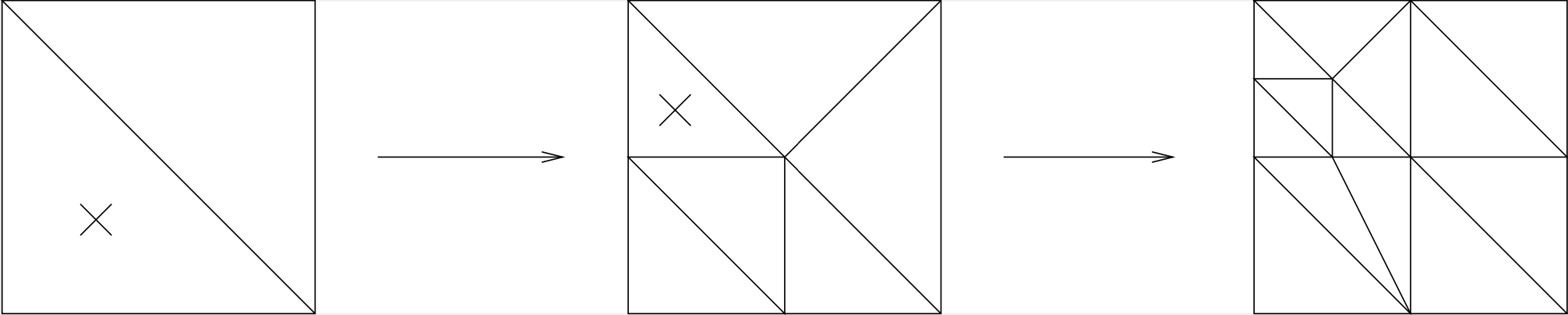
26.2.1. Red-Green Refinement

A marked element is split into four equivalent elements (called red refinement):

But, the obtained mesh is not regular. To avoid such irregular nodes, also neighboring elements must be split (called green closure):

If one continues to refine that way, the shape of the elements may get worse and worse:

A solution is that elements of the green closure will not be further refined. Instead, remove the green closure, and replace it by red refinement.

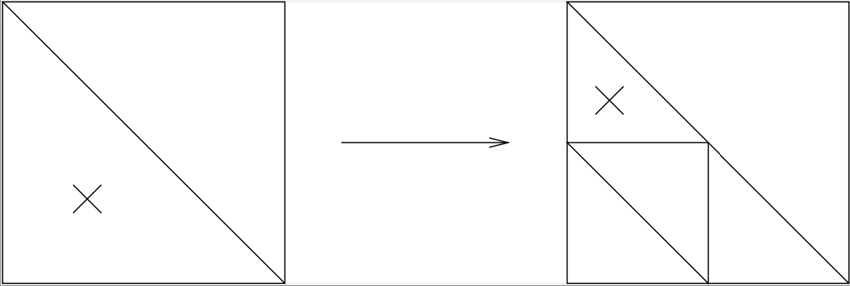
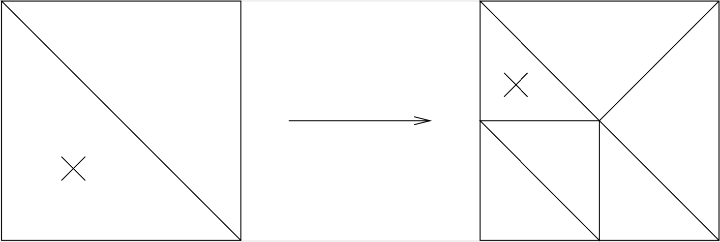
26.2.2. Marked edge bisection

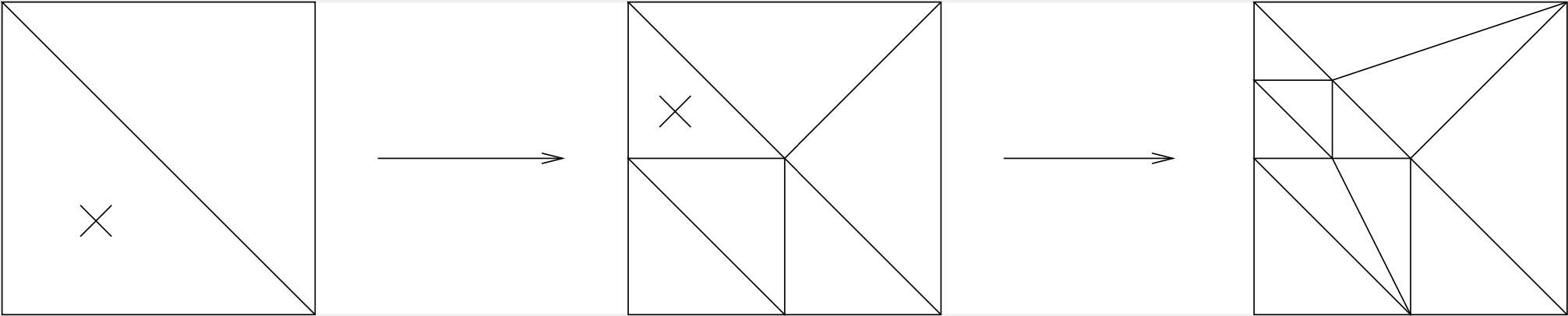
Each triangle has one marked edge. The triangle is only refined by cutting from the middle of the marked edge to the opposite vertex. The marked edges of the new triangles are the edges of the old triangle.

If there occurs an irregular node, then also the neighbor triangle must be refined.

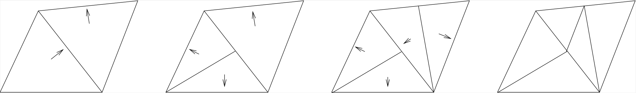
To ensure finite termination, one has to avoid cycles in the initial mesh. This can be obtained by first sorting the edges (e.g., by length), end then, always choose the largest edges as marked edge.

Both of these refinement algorithms are also possible in 3D.

26.3. Flux-recovery error estimates with NGSolve

from ngsolve import *
from netgen.occ import *
from ngsolve.webgui import Draw

We create a continuous, vector-valued GridFunction for the flux, and interpolate the finite element flux into it. Then we take element-wise the difference between the finite element flux, and the interpolated flux as element-wise error estimate. First we try for the Poisson equation, with constant \(1\), where the flux equals the gradient:

lshape = Line(1).Rotate(90).Line(1).Rotate(90).Line(2) \
    .Rotate(90).Line(2).Rotate(90).Line(1).Close().Face()
mesh = Mesh(OCCGeometry(lshape,dim=2).GenerateMesh(maxh=0.5))

fes = H1(mesh,order=3, autoupdate=True, dirichlet=".*")
u,v = fes.TnT()
a = BilinearForm(grad(u)*grad(v)*dx)
f = LinearForm(v*dx)
gfu = GridFunction(fes, autoupdate=True)
fesflux = VectorH1(mesh,order=3, autoupdate=True)
gfflux = GridFunction(fesflux, autoupdate=True)
lam = CF( 1 )
hist = []

def SolveEstimateMark():
    a.Assemble()
    f.Assemble()
    gfu.vec.data = a.mat.Inverse(fes.FreeDofs())*f.vec

    gfflux.Set(lam*grad(gfu))
    errest = Integrate ( lam*(1/lam*gfflux-grad(gfu))**2, mesh, element_wise=True)
    errmax = max(errest)
    hist.append ( (fes.ndof, sqrt(sum(errest)) ) )
    for i in range(mesh.GetNE(VOL)):
        mesh.SetRefinementFlag(ElementId(VOL,i), errest[i] > 0.25*errmax)

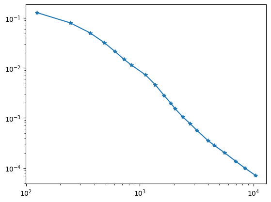
SolveEstimateMark()
while fes.ndof < 10000:
    mesh.Refine()
    SolveEstimateMark()

Draw (mesh);

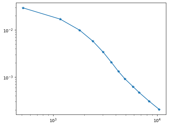
import matplotlib.pyplot as plt
plt.yscale('log')
plt.xscale('log')
plt.plot (*zip(*hist), '-*');

26.3.1. Variable coefficients

def MakeTwoMaterialMesh():
    r = Rectangle(2,2).Face()
    r.edges.name='dirichlet'
    inner = MoveTo(0.5,0.5).Rectangle(1,1).Face()
    outer = r-inner
    outer.faces.name="outer"
    inner.faces.name="inner"
    shape =Glue([outer,inner])
    return Mesh(OCCGeometry(shape,dim=2).GenerateMesh(maxh=0.3))

mesh = MakeTwoMaterialMesh()
fes = H1(mesh, order=3, autoupdate=True, dirichlet="dirichlet")
u,v = fes.TnT()
lam = mesh.MaterialCF( { "inner" : 5, "outer" : 1} )
a = BilinearForm(lam*grad(u)*grad(v)*dx)
f = LinearForm(v*dx("inner"))
gfu = GridFunction(fes, autoupdate=True)
fesflux = VectorH1(mesh,order=3, autoupdate=True)
gfflux = GridFunction(fesflux, autoupdate=True)

hist = []
SolveEstimateMark()
while fes.ndof < 10000:
    mesh.Refine()
    SolveEstimateMark()

Draw (mesh);

plt.yscale('log')
plt.xscale('log')
plt.plot (*zip(*hist), '-*');

We observe a very strong refinement along the material interface. This is unnecessary, since the solution is smooth on both sides, we only expect singularities at the corners. The problem is that the flux-averaging did an averaging of the full flux vector. The tangential component of it is not supposed to be continuous, and this it highly overestimates the error:

Draw (lam*grad(gfu)[0], mesh, order=2, min=-0.5, max=0.5);

Draw (gfflux[0], mesh, min=-0.5, max=0.5);

Draw (lam*grad(gfu)[0]-gfflux[0], mesh);

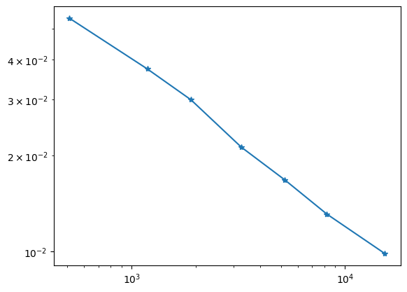
26.3.2. Flux recovery in \(H(\operatorname{div})\)

The over-refinement along the edges can be overcome by averaging only the normal component of the flux, since only this is supposed to be continuous. This we obtain by recovering the flux in an \(H(\operatorname{div})\) finite element space:

mesh = MakeTwoMaterialMesh()
fes = H1(mesh,order=3, autoupdate=True, dirichlet="dirichlet")
u,v = fes.TnT()
lam = mesh.MaterialCF( { "inner" : 5, "outer" : 1} )
a = BilinearForm(lam*grad(u)*grad(v)*dx)
f = LinearForm(v*dx("inner"))
gfu = GridFunction(fes, autoupdate=True)
fesflux = HDiv(mesh,order=3, autoupdate=True)
gfflux = GridFunction(fesflux, autoupdate=True)
hist=[]

SolveEstimateMark()
while fes.ndof < 10000:
    mesh.Refine()
    SolveEstimateMark()

Draw (mesh);

plt.yscale('log')
plt.xscale('log')
plt.plot (*zip(*hist), '-*');