71. Analysis of the Multigrid Iteration

We analyze the the condition number of the multigrid preconditioner. It uses the interplay of the smoothing iteration, and the coarse grid correction. The smoother is well suited for damping out high-frequency components of the error, while low frequency components can be well approximated on the coarse grid. We formulate the smoothing property satisfied by the smoother, and the approximation property due to the coarse-grid step.

We present the technique developed by Braess and Hackbusch, 83, which proves the optimal convergence of the V-cycle iteration, and even shows the improvement of convergence with increased number of smoothing-steps. However, it is based on the strong assumption of full elliptic regularity. There are many generalizations of the method and the analysis, like

• W-cycle: the coarse grid correction step is preformed twice

• variable V-cycle: the number of smoothing steps increase geometric for coarser levels

• non-nested setting: the coasre grid matrices only satisfy \(A_{l-1} \approx P_l^T A_l P_l\)

We refer to literature: Hackbusch 85, Bramble 93, Trottenberg et al 01

71.1. The Algorithm

The multigrid iteration matrix \(M_l\) and the multigrid preconditioner \(C_l\) are linked by

\[ M_l = I - C_l^{-1} A_l \]

They are recursively defined as

\[ M_l = (I-D_l^{-1} A_l)^m (I - P_l C_{l-1}^{-1} P_l^T A_l) (I -D_l^{-1} A_l)^m, \]

where \(C_0 := A_0\). The iteration matrix of the smoother \(D_l\) is

\[ S_l = I - D_l^{-1} A_l \]

We assume that the smoother \(D_l\) is spd, and scaled such that

\[ D_l \geq A_l \]

(in the sense of \(u^T D_l u \geq u^T A_l u \; \forall u\)) and thus

\[ \sigma (I - D_l^{-1} A_l) \subset [0,1] \]

We assume that the smoother is related to the \(L_2\)-norm as

\[ \| u_l \|_{D_l}^2 \preceq h_l^{-2} \| u_l \|_{L_2}^2. \]

This estimate holds for the (block-)Jacobi or symmetric (block-)Gauss-Seidel smoothers applied to finite element matrix of the Laplace operator.

71.2. The Approximation Property

We start with a function \(u_l\), and perform a coarse-grid correction step with exact coarse-grid solve:

\[ e_l = (I - P_l A_{l-1}^{-1} P_l^T A_l) u_l \]

If the coarse grid discretization is consistent, then this projection error \(e_l\) is small in \(L_2\)-norm:

\[ \| (I - P_l A_{l-1}^{-1} P_l^T A_l) u_l \|_{L_2} \preceq h \, \| u_l \|_{H^1} \]

We can prove this similar to the Aubin-Nitsche lemma using full elliptic regularity.

We introduce the coarse grid projector

\[ \Pi_{l-1} = P_l A_{l-1}^{-1} P_l^T A_l \]

Theorem [Approximation property] There holds with a constant \(C > 0\) independent of the refinement level:

\[ \forall \, u_l \in V_l : \qquad \| u_l - \Pi_{l-1} u_l \|_{D_l}^2 \leq C \, \| u_l - \Pi_{l-1} u_l \|_{A_l}^2 \]

Proof: We write \(u_l\) for the coefficient vector as well as for the corresponding finite element function in \(V_l\). For a given \(u_l\), define the \(A(.,.)\)-orthogonal projection \(u_{l-1} \in V_{l-1}\) via

\[ A(u_{l-1}, v_{l-1}) = A(u_l, v_{l-1}) \qquad \forall \, v_{l-1} \in V_{l-1} \]

The error \(e_l = u_l - u_{l-1}\) is \(A(.,.)\)-orthogonal to \(V_{l-1}\). As in the Aubin-Nitsche Lemma we define an artificial problem with the error as right hand side: find \(\varphi \in H^1\) such that

\[ A(\varphi, \psi) = (e_l, \psi)_{L_2} \qquad \forall \, \psi \in H^1. \]

Thanks to the regularity assumption the solution \(\varphi\) is in \(H^2\), and satisfies the regularity estimate

\[ \| \varphi \|_{H^2} \preceq \| e_l \|_{L_2} \]

Let \(\varphi_l\) and \(\varphi_{l-1}\) be the corresponding finite element solutions defined by \(A(\varphi_l, \psi_l) = (e_l, \psi_l)_{L_2}\), and \(A(\varphi_{l-1}, \psi_{l-1}) = (e_l, \psi_{l-1})_{L_2}\). They satisfy (by Cea’s Lemma):

\[\begin{eqnarray*} \| \varphi_l - \varphi_{l-1} \|_A & \leq & \| \varphi_l - \varphi \|_A + \| \varphi_{l-1} - \varphi \|_A \\ & \preceq & h \, \| \varphi \|_{H^2} \preceq h \, \| e \|_{L_2} \end{eqnarray*}\]

Now we use \(e_l = u_l - u_{l-1}\) as test-function, and use orthogonality several times:

\[\begin{eqnarray*} \| e_l \|_{L_2}^2 & = & (e_l, u_l - u_{l-1})_{L_2} \\ & = & A(\varphi_l, u_l) - A(\varphi_{l-1}, u_{l-1}) \\ & = & A(\varphi_l, u_l) - A(\varphi_{l-1}, u_l) \\ & = & A(\varphi_l - \varphi_{l-1}, u_l) \\ & = & A(\varphi_l - \varphi_{l-1}, u_l - u_{l-1}) \\ & \leq & \| \varphi_l - \varphi_{l-1} \|_A \, \| u_l - u_{l-1} \|_A \\ & \preceq & h \, \| e_l \|_{L_2} \| e_l \|_A \end{eqnarray*}\]

We have shown that

\[ h^{-1} \, \| u_l - u_{l-1} \|_{L_2} \preceq \| u_l - u_{l-1} \|_A \]

Since the smoother is dominated by the scaled \(L_2\)-norm there holds

\[ \| u_l - \Pi_{l-1} u_l \|_{D_l} \preceq h^{-1} \| u_l - \Pi_{l-1} u_l \|_{L_2} = h^{-1} \| u_l - u_{l-1} \|_{L_2}, \]

and the theorem is proven.

71.3. The Smothing Property

We have already seen that a basic iteration method with local preconditioners does not reduce the error well, i.e.

\[ \| S u \|_{A_l} \leq (1-c h^2) \| u \|_{A_l} \]

If \(\lambda \in \sigma(D_l^{-1} A_l)\), then

\[ 1 - \lambda \in \sigma (S). \]

Components in the eigen-spaces of eigen-values close to 1 are reduced well by the smoothing iteration, but error-components of eigen-values close to 0 are barely reduced. The large eigenvalues correspond to highly oscillating functions, smaller ones to smooth functions.

from ngsolve import *
from ngsolve.webgui import Draw
mesh = Mesh(unit_square.GenerateMesh(maxh=0.02))

fes = H1(mesh, order=1)
u,v = fes.TnT()
a = BilinearForm(grad(u)*grad(v)*dx).Assemble()
Dinv = a.mat.CreateSmoother()

gfu = GridFunction(fes)

# we start with a rough random function
gfu.vec.SetRandom()
Draw (gfu)

# performing some smoothing steps
for j in range(10):
    gfu.vec.data -= Dinv @ a.mat * gfu.vec
    
Draw (gfu);

The technique to quantify that is to use different norms for the input and the output of the smoothing iteration. We use a norm similar to the stronger \(H^2\) Sobolev-norm.

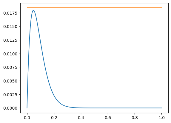
Theorem [Smoothing property]

\[ \| (I - D^{-1} A)^m u \|_{A D^{-1} A}^2 \leq \frac{1}{2 m e} \| u \|_A^2 \]

Proof: We use spectral theory. Expanding \(u\) in the eigensystem of \(A z = \lambda D z\) we can reformulate the inequality as

\[ \sum \lambda_i^2 (1 - \lambda_i)^{2m} u_i^2 \leq \frac{1}{2me} \sum \lambda_i u_i^2 \]

The estimate follows from estimating

\[ \max_{\lambda \in [0,1]} \lambda (1-\lambda)^{2m} \leq \frac{1}{2me}, \]

where the maximizer of the function on the left hand side is easily found and estimated by curve discussion.

from numpy import linspace
from math import exp
import matplotlib.pyplot as plt
%matplotlib inline
x = linspace(0,1,1000)
m=10
plt.plot(x, x*(1-x)**(2*m), x, [1/(2*m*exp(1)) for xi in x]);

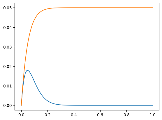
Lemma [Improved smoothing property]

\[ \| (I - D^{-1} A)^m u \|_{A D^{-1} A}^2 \leq \frac{1}{2m} \left( \| u \|_A^2 - \| (I-D^{-1} A)^m u \|_A^2 \right) \]

Proof: Very similar, we have to verify

\[ \lambda^2 (1-\lambda)^{2m} \leq \frac{1}{2m} \left( \lambda - \lambda (1-\lambda)^{2m} \right) \]

from numpy import linspace
import matplotlib.pyplot as plt
%matplotlib inline
x = linspace(0,1,100)
m=10
plt.plot(x, x**1*(1-x)**(2*m), x, 1/(2*m)*(1-(1-x)**(2*m)));

71.4. Optimal convergence of the \(V\)-cycle

We can now combine these properties to analyze the multigrid iteration:

Theorem: Assume that the approximation property (with constant \(C\)) and the smoothing property are satisfied. Then there holds

\[ \| M_l \|_A \leq \delta \]

with

\[ \delta = \frac{C}{C+2m} < 1. \]

Proof: We prove the claim per induction. For \(l=0\) there holds \(M_0 = 0\).

From \(M_{l-1} = I - C_{l-1}^{-1} A_{l-1}\) there follows \(C_{l-1}^{-1} = (I - M_{l-1}) A_{l-1}^{-1}\).

We carefully split the iteration matrix into an iteration matrix with exact coarse grid solve, plus its perturbation:

\[\begin{eqnarray*} (M_l u, u)_{A_l} & = & \big( S_l^m (I - P_l C_{l-1}^{-1} P_l^T A_l) S_l^m u, u \big)_{A_l} \\ & = & \big( (I - P_l C_{l-1}^{-1} P_l^T A_l) S_l^m u, S_l^m u \big)_{A_l} \\ & = & \big( (I - P_l (I-M_{l-1}) A_{l-1}^{-1} P_l^T A_l) S_l^m u, S_l^m u)_{A_l} \\ & = & ((I-P_l A_{l-1}^{-1} P_l^T A_l) S_l^m u, S_l^m u)_{A_l} \\ & & \quad + (P_l M_{l-1} A_{l-1}^{-1} P_l^T A_l S_l^m u, S_l^m u)_{A_l} \\ & = & ( (I-\Pi_{l-1}) S_l^m u, S_l^m u)_{A_l} \\ & & + (M_{l-1} A_{l-1}^{-1} P_l^T A_l S_l^m u, A_{l-1}^{-1} P_l^T A_l S_l^m u)_{A_{l-1}} \end{eqnarray*}\]

We use the induction assumption \(\| M_{l-1} \|_{A_{l-1}} \leq \delta\) for the second term:

\[\begin{eqnarray*} (M_l u, u)_{A_l} & \leq & (I-\Pi_{l-1}) S_l^m u, S_l^m u)_{A_l}^2 + \delta \, ( \Pi_{l-1} S_l^m u, S_l^m u)_{A_l} \\ & = & (1-\delta) \big( (I-\Pi_{l-1}) S_l^m u, S_l^m u \big)_A^2 + \delta \, ( S_l^m u, S_l^m u) \end{eqnarray*}\]

We continue with the first term, apply Cauchy-Schwarz for the \((.,.)_{D_l}\) inner product, and use approximation and smoothing properties:

\[\begin{eqnarray*} \big( (I-\Pi_{l-1}) S_l^m u, S_l^m u \big)_{A_l} & = & \| (I-\Pi_{l-1}) S_l^m u \|_{A_l}^2 \\ & = & \big( (I-\Pi_{l-1}) S_l^m u, D_l^{-1} A_l S_l^m u \big)_{D_l} \\ & \leq & \| (I-\Pi_{l-1}) S_l^m u \|_{D_l} \| S_l^m u \|_{AD^{-1} A} \\ & \leq & \sqrt{C} \| (I-\Pi_{l-1}) S_l^m u \|_{A_l} \sqrt{\frac{1}{2m} \big( \| u \|_{A_l}^2 - \| S_l^m u \|_{A_l}^2 \big)} \end{eqnarray*}\]

Dividing by one factor \(\| (I-\Pi_{l-1}) S_l^m u \|_{A_l}\) we get

\[ \| (I-\Pi_{l-1}) S_l^m u \|_{A_l}^2 \leq \frac{C}{2m} \big( \| u \|_{A_l}^2 - \| S_l^m u \|_{A_l}^2 \big) \]

Combining both estimates and using \(\| S_l u \|_{A_l} \leq \|u \|_{A_l}\) we get

\[\begin{eqnarray*} (M_l u, u)_A & \leq & (1-\delta) \frac{C}{2m} ( \| u \|_{A_l}^2 - \| S_l^m u \|_{A_l}^2 ) + \delta \, \| S_l^m u \|_{A_l}^2 \\ & \leq & \frac{(1-\delta) C}{2m} \| u \|_A^2 + \big( \delta - \frac{(1-\delta) C}{2m} \big) \| S_l^m u \|_A^2 \\ & \leq & \frac{(1-\delta) C}{2m} \| u \|_{A_l}^2 + \big( \delta - \frac{(1-\delta) C}{2m} \big) \| u \|_{A_l}^2 \\ & = & \delta \, \| u \|_{A_l}^2 \end{eqnarray*}\]

We used that by the choice of \(\delta\) the factor \(\delta - \frac{(1-\delta) C}{2m}\) is positive. The proof is complete.