17.4. Coding the Implicit Euler method#
In every time-step we have to solve for the new value \(y^{n+1}\):
The function \(f : {\mathbb R}^n \rightarrow {\mathbb R}^n\) is the right-hand side of the ODE, which has been brought into autonomous form.
For the current time-step we rename \(y_i\) and \(y_{i+1}\) to \(y_{\text{old}}\) and \(y\), and rewrite the equation as
We use our function algebra to build this composed function m_equ, and throw it into the Newton solver.
If we make the time-step not too large, the value \(y^n\) of the old time-step is a good starting value.
To express that the independent variable is \(y^{n+1}\), we create an IdentityFunction. The old
value \(y_{\text{old}}\) is a constant, represented as ConstantFunction.
In every time-step we reset the value for \(y_{\text{old}}\).
The time-step \(\tau\) itself goes as Parameter into the function algebra. Such a parameter can be set and changed later.
Then the implementation of the implicit Euler method looks like:
class ImplicitEuler : public TimeStepper
{
  std::shared_ptr<NonlinearFunction> m_equ;
  std::shared_ptr<Parameter> m_tau;
  std::shared_ptr<ConstantFunction> m_yold;
public:
  ImplicitEuler(std::shared_ptr<NonlinearFunction> rhs)
    : TimeStepper(rhs), m_tau(std::make_shared<Parameter>(0.0))
  {
    m_yold = std::make_shared<ConstantFunction>(rhs->dimX());
    auto ynew = std::make_shared<IdentityFunction>(rhs->dimX());
    m_equ = ynew - m_yold - m_tau * m_rhs;
  }

  void DoStep(double tau, VectorView<double> y) override
  {
    m_yold->set(y);
    m_tau->set(tau);
    NewtonSolver(m_equ, y);
  }
};
17.4.1. Excercises#
Try the implicit Euler method for the mass-pring system
Implement the Crank-Nicolson method.
Compare the results of the mass-spring system for these three methods, and various time-steps. What do you oberve?
Model an electric network by an ODE. Bring it to autonomous form. Solve the ODE numerically for various parameters with the three methods, and various time-steps.
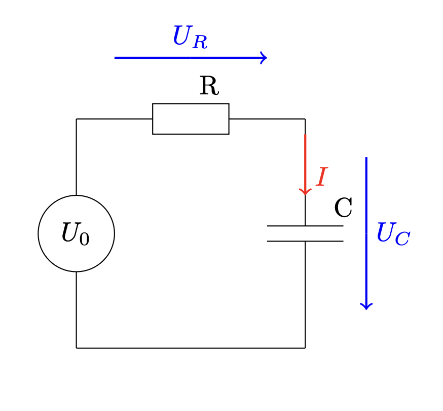
Voltage source \(U_0(t) = \cos(100 \pi t)\), \(R = C = 1\) or \(R = 100, C = 10^{-6}\).
Ohm’s law for a resistor \(R\) with resistivity \(R\):
\[ U = R I \]Equation for a capacitor \(C\) with capacity \(C\):
\[ I = C \frac{dU }{dt} \]Kirchhoff’s laws:
Currents in a node sum up to zero. Thus we have a constant current along the loop.
Voltages around a loop sum up to zero. This gives:
\[ U_0 = U_R + U_C \]
Together:
\[ U_C(t) + R C \frac{dU_C}{dt}(t) = U_0(t) \]Use initial condition for voltage at capacitor \(U_C(t_0) = 0\), for \(t_0=0\).
17.4.2. Stability function#
The observations you made can be explained by the stability function of the method.
An ODE \(y^\prime(t) = A y(t)\) with \(A \in {\mathbb R}^n\) diagonizable can be brought to \(n\) scalar ODEs
where \(\lambda_i\) are eigenvalues of \(A\). If \(\lambda_i\) has negative (non-positive) real part, the solution is decaying (non-increasing). Skip index \(i\).
The explicit Euler method with time-step \(h\) leads to
the implicit Euler method to
and the Crank-Nicolson to
The stability function \(g(\cdot)\) of a method is defined such that
These are for the explicit Euler, the implicit Euler, and the Crank-Nicolson:
The domain of stability is
What is
If Re\((\lambda) \leq 0\), then \(\tau \lambda\) is always in the domain of stability of the implicit Euler, and of the Crank-Nicolson. This property of an method is called \(A\)-stability. The explicit Euler leads to (quickly) increasing numerical solutions if \(\tau\) is not small enough.
If \(\lim_{z \rightarrow -\infty} g(z) = 0\), quickly decaying solutions lead to quickly decaying numerical solutions. This is the case for the implicit Euler, but not for the Crank-Nicolson. This property is called \(L\)-stability. One observes (slowly decreasing) oscillations with the CR - method when \(-\tau \lambda\) is large.