23.4. NACA airfoil

The NACA airfoil series is a set of standardized airfoil shapes, which became widely used in the design of aircraft wings. See https://en.wikipedia.org/wiki/NACA_airfoil

We use the Python code naca.py by Dirk Gorissen, and adapted by Xaver Mooslechner and Edoardo Bonetti to Netgen-OCC geometry.

from ngsolve import *
from netgen.occ import *
from ngsolve.webgui import Draw
import matplotlib.pyplot as plt
from naca import naca4
import numpy as np

def occ_naca_profile(alpha = 12, h=0.03):

    xs, ys = naca4("2412", 600)
    pnts = list (zip ( xs, ys, (0,)*len(xs) ))
    
    curve = Wire(SplineApproximation(pnts))
    wing = Face(curve)
    wing.edges.name = "wing"
    wing.edges.maxh = h

    rect = Rectangle(6, 2).Face().Move((-1.5, -1, 0))
    rect.edges.name = "wall"
    rect.edges.Min(X).name="inlet"
    rect.edges.Max(X).name = "outlet"
    wing = wing.Rotate(Axis((0,0,0), Z),-alpha)
    air =  rect - wing
    
    return air

with TaskManager():
    mesh = Mesh(OCCGeometry(occ_naca_profile(alpha=12, h=0.01), dim=2).GenerateMesh(maxh=0.1))
    mesh.Curve(3)
Draw(mesh);
print ("ne = ", mesh.GetNE(VOL))

ne =  4155

def NavierStokes(R, tau , tend):

    V = VectorH1(mesh, order=1, dirichlet="wall|wing|inlet")
    V.SetOrder(TRIG, 3)
    V.Update()

    Q = H1(mesh, order=1)

    X = V*Q

    drag_x_test = GridFunction(X)
    drag_x_test.components[0].Set(CoefficientFunction(
        (-1, 0)), definedon=mesh.Boundaries("wing"))
    drag_y_test = GridFunction(X)
    drag_y_test.components[0].Set(CoefficientFunction(
        (0, -1)), definedon=mesh.Boundaries("wing"))
    time_vals, drag_x_vals, drag_y_vals = [], [], []


    u, p = X.TrialFunction()
    v, q = X.TestFunction()

    stokes = 1/R*InnerProduct(grad(u), grad(v))+div(u)*q+div(v)*p - 1e-10*p*q
    a = BilinearForm(X, symmetric=True)
    a += stokes*dx
    a.Assemble()

    # nothing here ...
    f = LinearForm(X)
    f.Assemble()

    # gridfunction for the solution
    gfu = GridFunction(X)

    # parabolic inflow at inlet:
    uin = CoefficientFunction(((1-y)*(1+y), 0))
    gfu.components[0].Set(uin, definedon=mesh.Boundaries("inlet"))

    # solve Stokes problem for initial conditions:
    inv_stokes = a.mat.Inverse(X.FreeDofs())

    res = f.vec.CreateVector()
    res.data = f.vec - a.mat*gfu.vec
    gfu.vec.data += inv_stokes * res


    # matrix for implicit Euler
    mstar = BilinearForm(X, symmetric=True)
    mstar += (u*v + tau*stokes)*dx
    mstar.Assemble()
    inv = mstar.mat.Inverse(X.FreeDofs(), inverse="sparsecholesky")

    # the non-linear term
    conv = BilinearForm(X, nonassemble=True)
    conv += (grad(u) * u) * v * dx

    # for visualization
    sceneu = Draw(Norm(gfu.components[0]), mesh, "velocity", sd=3)    
    #scenep = Draw(Norm(gfu.components[1]), mesh, "pressure", sd=3)


    # implicit Euler/explicit Euler splitting method:
    t = 0
    i = 0
    with TaskManager():
        while t < tend:
            # print("t=", t, end="\r")

            conv.Apply(gfu.vec, res)
            res.data += a.mat*gfu.vec
            gfu.vec.data -= tau * inv * res

            time_vals.append(t)
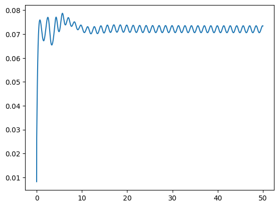
            drag_x_vals.append(InnerProduct(res, drag_x_test.vec))
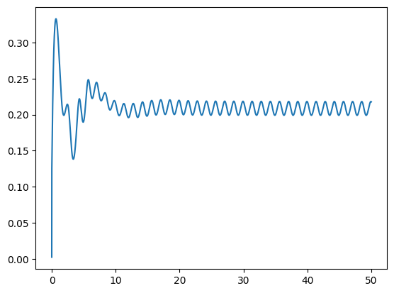
            drag_y_vals.append(InnerProduct(res, drag_y_test.vec))
            t = t + tau
            i = i+1

            if i % 30 == 0:
                sceneu.Redraw()
                #scenep.Redraw()

    
    plt.plot(time_vals, drag_x_vals)
    plt.show()
    plt.plot(time_vals, drag_y_vals)
    plt.show()

R = 1800
tau = 2e-3
tend = 50

NavierStokes(R, tau, tend)