24.1. Magnetostics

We consider the special case of stationary magnetic fields.

A magnetic field is caused by an electric current. We suppose that a current density

\[ j \in [L_2(\Omega)]^3 \]

is given. Stationary currents do not have sources, i.e., \(\operatorname{div} \, j = 0\). Current through a wire causes a magnetic field around the wire:

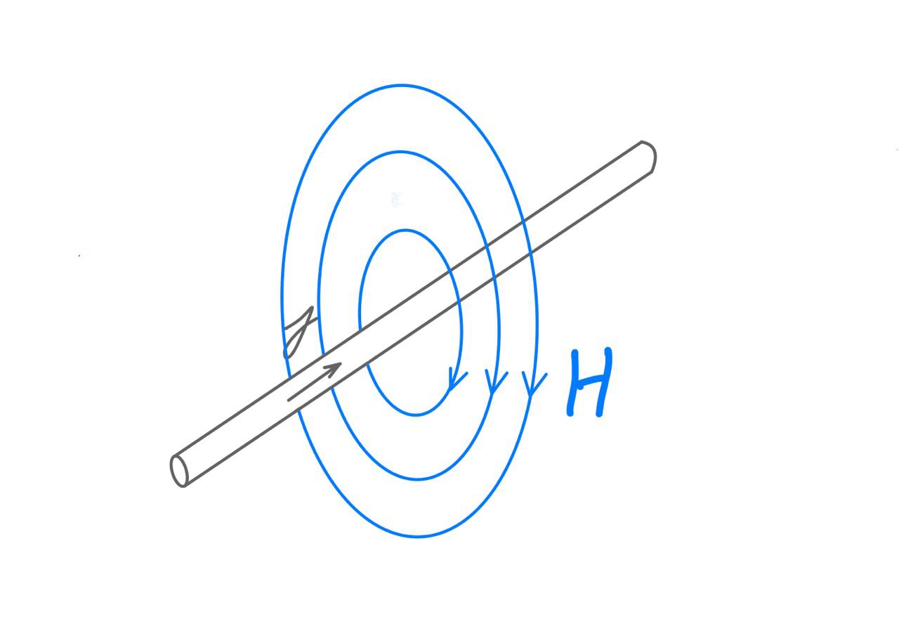
The involved (unknown) fields are

• The magnetic flux \(B\) (in German: Induktion). The flux is free of sources, i.e.,

\[ \operatorname{div} \, B = 0. \]

• The magnetic field intensity \(H\) (in German: magnetische Feldstärke). The field is related to the current density by Ampère’s law:

\[ \int_S j \cdot n \, ds = \int_{\partial S} H \cdot \tau \qquad \forall \; \mbox{Surfaces } S \]

By Stokes’ Theorem \(\int_{\partial S} H \cdot \tau = \int_S \operatorname{curl} H \cdot n \, ds\), one obtains Ampère’s law in differential form:

\[ \operatorname{curl} \, H = j \]

The differential operator is \(\operatorname{curl} = \operatorname {rot} = \nabla \times\). Both fields are related by a material law. The coefficient \(\mu\) is called permeability:

\[ B = \mu H \]

The coefficient \(\mu\) is \(10^3\) to \(10^4\) times larger in iron (and other ferro-magnetic metals) as in most other media (air). In a larger range, the function \(B(H)\) is also highly non-linear.

Collecting the equations we have

\[ \operatorname{div} \, B = 0 \qquad B = \mu H \qquad \operatorname{curl} \, H = j \]

In principle, Maxwell equations are valid in the whole \(\mathbb{R}^3\). For simulation, we have to truncate the domain and have to introduce artificial boundary conditions.

Since \(\operatorname{div} B = 0\), and the domain \({\mathbb R}^3\) is simply connected, we may introduce a vector potential \(A\) such that

\[ B = \operatorname{curl} \, A. \]

Inserting the vector-potential into the system of equations, one obtains the second order equation

(24.1)\[\begin{equation} \operatorname{curl} \, \mu^{-1} \operatorname{curl} A = j. \end{equation}\]

The two original fields \(B\) and \(H\) can be obtained from the vector potential \(A\).

The vector-potential \(A\) is not uniquely defined. One may add a gradient field to \(A\), and the equation is still true. To obtain a unique solution, the so called Coloumb-Gauging can be applied:

(24.2)\[\begin{equation} \operatorname{div} \, A = 0. \end{equation}\]

24.1.1. Variational formulation

As usual, we go over to the weak form. Both equations together become: Find \(A\) such that

\[ \int_\Omega \mu^{-1} \operatorname{curl} A \, \operatorname{curl} v \, dx = \int_\Omega j \cdot v \, dx \qquad \forall \, v \in ? \]

and

\[ \int_\Omega A \cdot \nabla \psi \, dx = 0. \]

We want to choose the same space for \(A\) and the according test functions \(v\). But, then we have more equations than unknowns. The system is still solvable, since we have made the assumption \(\operatorname{div} \, j = 0\), and thus \(j\) is in the range of the \(\operatorname{curl}\)- operator. To obtain a symmetric system, we add a new scalar variable \(\varphi\). The problem is now: Find \(A \in V = ?\) and \(\varphi \in Q = H^1 / \mathbb{R}\) such that

(24.3)\[\begin{equation} \begin{array}{ccccll} \int \mu^{-1} \operatorname{curl} A \, \cdot \operatorname{curl} v \, dx & + & \int \nabla \varphi \cdot v \, dx & = & \int j \cdot v \, dx \qquad & \forall \, v \in V \\[0.5em] \int A \cdot \nabla \psi \, dx & & & = & 0 & \forall \, \psi \in Q \end{array} \end{equation}\]

24.1.2. Gauging by regularization

Instead of posing the div-free constraint by a Lagrange parameter, one often solves the regularized problem with a small regularization parameter \(\varepsilon\): Find \(A \in V\):

\[ \int \mu^{-1} \operatorname{curl} A^{\varepsilon} \, \cdot \operatorname{curl} v \, dx + \varepsilon \int A^{\varepsilon} \cdot v \, dx = \int j \cdot v \, dx \qquad \forall \, v \in V \]

If we apply test-functions \(v = \nabla \psi\), use \(\operatorname{curl} \nabla = 0\), and \(\int j \cdot \nabla \psi = 0\), we obtain

\[ \int A^\varepsilon \cdot \nabla \psi \, dx = 0 \qquad \forall \psi \in H^1 \]

One can show that \(A^\varepsilon \rightarrow A\) for \(\varepsilon \rightarrow 0\).

For \(\varepsilon = 0\) the bilinear-form is a large null-space \(V_0 = \nabla H^1\), and the finite element matrix is only positive semi-definite. By regularization, the zero-eigenvalues are replaced by small positive eigenvalues. Since the right hand side \(\int j v dx\) is orthogonal to the null-space, the right hand side vector is in the range of the semi-definite matrix.