35. Multipole basis functions#
The building blocks for multipole expansions are spherical harmonics, as well as spherical Bessel and Hankel functions. They arise from separation of variables of the Helmholtz operator, in spherical coordinates. We only state the results, for derivation we refer to the cited literature.
We define singular and regular multipoles as the following series:
where
\(r = |x|\), \(\hat x = x/r\)
\(a_{nm}\) and \(b_{nm}\) are complex-valued expansion coefficients
\(h_n\) and \(j_n\) are spherical Hankel and Bessel functions, see below
\(Y_n^m\) are so called spherical harmonics, an orthogonal basis on the sphere, see below
35.1. Spherical harmonics#
For \(n = 0, 1, 2, \ldots\) and \(-n \leq m \leq n\) we define
with the associated Legendre functions \(P_n^m\), for \(m \leq n\) are defined as: (TODO)
We call \(n\) the degree, and \(m\) the order. Spherical harmonics with the same degree are combined with the same Hankel or Bessel functions.
The polar angle \(\theta \in [0,\pi]\) and the azimuthal angle \(\varphi \in [-\pi, \pi)\) are defined such that
from ngsolve import *
from netgen.occ import *
from ngsolve.webgui import Draw

sp = Sphere((0,0,0),1).faces[0]
mesh = Mesh(OCCGeometry(sp).GenerateMesh(maxh=0.2)).Curve(3)
from ngsolve.bem import SphericalHarmonicsCF
We draw the spherical harmonics \(Y_n^m\) of degree \(n=8\) and order \(m=3\). We see that \(n\) gives the number of roots in the polar direction, and \(2m\) is the number of roots in azimuthal direction:
shcf = SphericalHarmonicsCF(10)
shcf.sh[4,2] = 1
Draw (shcf, mesh, animate_complex=True, order=3, euler_angles=[-27,-7,6]);
These functions form an \(L_2\)-orthonormal basis on the sphere.
35.2. Spherical Bessel and Hankel functions#
The spherical Hankel functions are expressed via spherical Bessel functions as
so we focus on the Bessel functions in the following (precisely, we are using Hankel functions of the first kind \(h_n^{(1)}\))
We define spherical Bessel functions of the first kind
and
with special setting \(j_0(0) = 1\) and \(j_n(0) = 0\) for \(n \geq 1\).
and of the second kind:
and
Some facts:
Bessel functions of the first kind, \(j_n\), are smooth up to \(x = 0\).
Bessel functions of the second kind, \(y_n\), have singularities at \(x=0\) of order \(n\).
Both satisfy the same recurrence relations
35.2.1. Behavior for large \(n\) and \(x\)#
We want to compute with large coefficients \(n\) and large arguments \(x\). Then the evaluation by the recurrences becomes unstable (for the \(j_n\)), and it requires sophisticated algorithms.
Looking hat these functions at large index \(n\) shows the interesting behavior:
from scipy.special import spherical_jn, spherical_yn
import matplotlib.pyplot as plt
import numpy as np

x = np.linspace(0,200, 1000)
plt.ylim(-1.8,1.8)
plt.plot (x, x*spherical_jn(50, x))
with np.errstate(invalid='ignore'):
    plt.plot (x, x*spherical_yn(50, x));
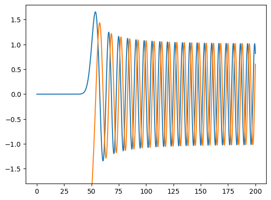
For \(x > n\), both Bessel functions are oscillating, with amplitudes decreasing like \(1/x\). For \(x < n\), the \(j_n\) are extremely small, while \(y_n\) are extremely large. This explains the unstable behaviour of the recursion for the \(j_n\). We use the recusion in \(n\). For \(n \leq x\), the \(j_n\) are \(O(1)\), but for \(n > x\) they become very small. Unavoidable roundoff errors for small \(n\) lead to huge relative errors for the higher \(n\). High quality implementations compute the recurrence backward, where it is stable, and also take care of leaving the range of floating point numbers, see e.g. the implementation from FMM3D on github