Approximation of functions

20.3. Approximation of functions#

In this section we investigate how well we can approximate given functions by finite element functions. We compare various opportunities to project a function into the fe space:

Interpolation:
The function is first interpolated in element vertices.
In the second step the degrees of freedom on the element edges are set, which could also be done by interpolation in nodes on the edges. An alternative is to project the function on the edges by solving a 1D variations problem for each edge, and keeping the vertex values unchanged.
As a third step, the interior degrees of freedom are set. Possibly also by interpolation, but here the choice of stable interpolation points on simplicial elements is unclear. The alternative is to solve an element-wise Dirichlet-problem. In NGSolve, this is obtained via
```
gfu.Interpolate(ugiven)
```
Interpolation is implemented for many finite elements spaces, but not for all.
Global $L_2$-projection:
This option allows to approximate discontinuous functions. However, one needs to solve a global linear system to determine the expansion coefficients. In NGSolve, one can formulate a variational problem to realize the $L_2$-projection.
Local $L_2$-projection:
In a first step, one computes the element-wise $L_2$-projection for each individual element. To obtain a continuous function, one performs arithmetic averaging of values in vertices and on edges. This is obtained using
```
gfu.Set(ugiven)
```
The local $L_2$-projection is implemented generically for all spaces where it makes sense (i.e. provide element-wise basis functions).

20.3.1. Smooth functions#

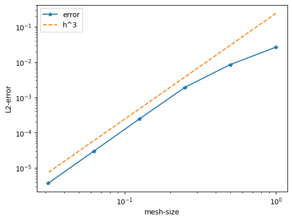
We approximate smooth functions. We expect convergence rates

\[ \| u - \Pi_h u \|_{L_2} \leq c h^{k+1} \| u \|_{H^{k+1}} \]

for finite elements of order $k$. The constant $c$ is independent of the mesh-size $h$, but depends on the order $k$.

from ngsolve import *
from ngsolve.webgui import Draw

def ComputeError (func, order, maxh=0.3, reflevels=0):
    mesh = Mesh(unit_square.GenerateMesh(maxh=maxh))
    for l in range(reflevels):
        mesh.Refine()
    fes = H1(mesh, order=order)
    gfu = GridFunction(fes)
    gfu.Set (func)

    err = sqrt(Integrate( (func-gfu)**2, mesh, order=2*order+4))
    return fes.ndof, err

ComputeError (x*x, order=1, maxh=0.5, reflevels=4)

(833, 0.0001751686634605984)

errors = []
hs = []
func = sin(pi*x)
for l in range(6):
    ndof, err = ComputeError (func, order=2, maxh=1, reflevels=l)
    errors.append(err)
    hs.append(1/2**l)

import matplotlib.pyplot as plt
plt.xscale('log')
plt.yscale('log')
plt.xlabel('mesh-size')
plt.ylabel('L2-error')
plt.plot (hs, errors, '-*', label="error")
plt.plot ( [hs[0], hs[-1]], [2*errors[-1]*(hs[0]/hs[-1])**3,2*errors[-1]], '--', label="h^3")
plt.legend();

../../_images/0aa504e2a342544440c61816eaeed042951857bff8b5b86971e26d7ce05d2d81.png

20.3.2. Exercises#

20.3.2.1. Study convergence depending on polynomial order.#

It’s fair to plot the error over number of degrees of freedom.

20.3.2.2. Study convergence in the $H^1$-semi-norm.#

Measure the interpolation error $\| \nabla (u - \Pi_h u) \|$. Here, symbolic differentiation of the given function is useful:

func = sin(10*x*y)
print ("func=\n", func)
gradfunc = CF( (func.Diff(x), func.Diff(y))) # make vectorial coefficient-function of partial derivatives
print ("gradient=\n", gradfunc)

func=
 coef unary operation 'sin', real
  coef binary operation '*', real
    coef scale 10, real
      coef coordinate x, real
    coef coordinate y, real

gradient=
 coef unary operation ' ', real, dim=2
  coef VectorialCoefficientFunction, real, dim=2
    coef binary operation '*', real
      coef unary operation 'cos', real
        coef binary operation '*', real
          coef scale 10, real
            coef coordinate x, real
          coef coordinate y, real
      coef binary operation '*', real
        coef coordinate y, real
        coef scale 10, real
          coef 1, real
    coef binary operation '*', real
      coef unary operation 'cos', real
        coef binary operation '*', real
          coef scale 10, real
            coef coordinate x, real
          coef coordinate y, real
      coef binary operation '*', real
        coef scale 10, real
          coef coordinate x, real
        coef 1, real

20.3.2.3. Functions with singularities#

Consider functions with singularities like $\sqrt{x^2+y^2}^\alpha$

Here, geometric mesh refinement towards the singular corner may help:

from netgen.occ import *
square = Rectangle(1,1).Face()
square.vertices.Min(X+Y).hpref = 1
mesh = Mesh(OCCGeometry(square, dim=2).GenerateMesh(maxh=0.3))
mesh.RefineHP(4, factor=0.25)
Draw (mesh);

20.3.2.4. Discontinuous functions#

Consider functions like $$ f(x,y) = \left\{ \begin{array}{cc} 1 & \text{for } (x-0.5)^2+(y-0.5)^2 < 0.3^2 \\ 0 & \text{else} \end{array} \right., $$ or functions with a kink like $\max {0.3^2-(x-0.5)^2-(y-0.5)^2, 0 }$. Plot the interpolated functions.

mesh = Mesh(unit_square.GenerateMesh(maxh=0.05))
func = IfPos( (x-0.5)**2 + (y-0.5)**2 - 0.3**2, 0, 1)
Draw (func, mesh, order=10);   # use 10^2 points per element for plotting

Does it help to resolve the discontinuity by the geometry?

When should we replace H1 by L2 ?

square = Rectangle(1,1).Face()
circ = Circle((0.5, 0.5), 0.3).Face()
outer = square-circ
circ.faces.name="inner"
outer.faces.name="outer"
shape = Glue([outer,circ])
Draw (shape)
mesh = Mesh(OCCGeometry(shape, dim=2).GenerateMesh(maxh=0.05)).Curve(1)
Draw (mesh);