23. Gauss-Bonnet Theorem#
The Gauss-Bonnet theorem relates the curvature of a surface \(\mathcal{S}\) with a topological quantity. For closed smooth surfaces there holds with the Gauss curvature \(K\)
where \(\chi_{\mathcal{S}}\) is the Euler characteristic of the surface. For a triangulation of \(\mathcal{S}\) the Euler characteristic can be computed by \(\chi_{\mathcal{S}}=\# T-\# E + \# V\), i.e., the number of triangles minus numer of edges plus number of vertices. It is related to the genus \(g\) of a connected closed surface (‘’number of holes’’). For orientable surfaces there holds \(\chi_{\mathcal{S}}=2-2g\).
from ngsolve import *
from netgen.occ import *
from ngsolve.webgui import Draw

order = 4


def GaussCurv():
    nsurf = specialcf.normal(3)
    return Cof(Grad(nsurf)) * nsurf * nsurf
For a sphere \(K=\frac{1}{R^2}\) and its Euler characteristic is \(2\) (genus \(g=0\)).
sphere = Sphere((0, 0, 0), 3).faces[0]
mesh = Mesh(OCCGeometry(sphere).GenerateMesh(maxh=0.4)).Curve(order)
Draw(mesh)
print(
    "int_S K =",
    Integrate(GaussCurv() * ds, mesh),
    " = ",
    2 * pi * 2,
    " = 2*pi*(#T-#E+#V) = ",
    2 * pi * (mesh.nface - mesh.nedge + mesh.nv),
)
int_S K = 12.566702932823253 = 12.566370614359172 = 2*pi*(#T-#E+#V) = 12.566370614359172
An ellipsoid is topologically equivalent to a sphere. Therefore we expect it to have the same Euler characteristic.
ell = Ellipsoid(Axes((0, 0, 0), X, Y), 0.75, 1 / 2, 1 / 3).faces[0]
mesh = Mesh(OCCGeometry(ell).GenerateMesh(maxh=0.07)).Curve(order)
Draw(mesh)
print(
    "int_S K =",
    Integrate(GaussCurv() * ds, mesh),
    " = ",
    2 * pi * 2,
    " = 2*pi*(#T-#E+#V) = ",
    2 * pi * (mesh.nface - mesh.nedge + mesh.nv),
)
int_S K = 12.572887858890471 = 12.566370614359172 = 2*pi*(#T-#E+#V) = 12.566370614359172
A torus has Euler characteristic \(\chi_{\mathcal{S}}=0\), genus \(g=1\) as it has one hole.
circ = WorkPlane(Axes((3, 0, 0), -Y, X)).Circle(1).Face()
torus = Revolve(circ, Axis((0, 0, 0), (0, 0, 1)), 360)
torus.faces.name = "torus"
mesh = Mesh(OCCGeometry(torus.faces[0]).GenerateMesh(maxh=0.8)).Curve(order)
Draw(mesh)
print(
    "int_S K =",
    Integrate(GaussCurv() * ds, mesh),
    " = ",
    0,
    " = 2*pi*(#T-#E+#V) = ",
    2 * pi * (mesh.nface - mesh.nedge + mesh.nv),
)
int_S K = 0.01739265812602292 = 0 = 2*pi*(#T-#E+#V) = 0.0
If we combine two tori the Euler characteristic changes to \(-2\).
torus2 = Translation((6.5, 0, 0))(torus)
torus2.faces.name = "torus2"
two_torus = Glue((torus2 - torus).faces["torus2"] + (torus - torus2).faces["torus"])
mesh = Mesh(OCCGeometry(two_torus).GenerateMesh(maxh=1)).Curve(order)
Draw(mesh)
print(
    "int_S K =",
    Integrate(GaussCurv() * ds, mesh),
    " = ",
    2 * pi * (2 - 4),
    " = 2*pi*(#T-#E+#V) = ",
    2 * pi * (mesh.nface - mesh.nedge + mesh.nv),
)
int_S K = -4.099937349046166 = -12.566370614359172 = 2*pi*(#T-#E+#V) = -12.566370614359172
The computation with number of triangles, edges, and vertices matches, but the integral of the Gauss curvature does not. Why?
The generated surface is not smooth at the interface!
23.1. Gauss-Bonnet for non-closed and non-smooth surfaces#
For non-closed and non-smooth surfaces the Gauss-Bonnet theorem is of the form
We have to include the geodesic curvature at the non-smooth interface from both sides of the tori to repair the results.
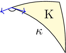
We recall that with the tangent vector \(t\) and co-normal vector \(\mu\) the geodesic curvature is given by
mu = Cross(specialcf.normal(3), specialcf.tangential(3))
edgecurve = specialcf.EdgeCurvature(3)  # nabla_t t

print(
    "int_S K + int_{dS} k_g =",
    Integrate(GaussCurv() * ds, mesh),
    " + ",
    Integrate(-edgecurve * mu * ds(element_boundary=True), mesh),
    " = ",
    Integrate(GaussCurv() * ds - edgecurve * mu * ds(element_boundary=True), mesh),
)
int_S K + int_{dS} k_g = -4.099937349046166 + -8.477058185545866 = -12.576995534592033
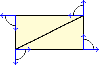
Next, consider a flat rectangle. It is topologically equivalent to the half-sphere. Thus \(\chi_{\mathcal{S}}=1\). But it has zero Gauss and geodesic curvature.
Now we need to consider also the non-smooth boundary at the four vertices. Each of them has angle \(\frac{\pi}{2}\) and thus some up to \(2\pi\) such that Gauss-Bonnet is again fulfilled.
mesh = Mesh(OCCGeometry(Rectangle(2, 1).Face(), dim=3).GenerateMesh(maxh=2))
Draw(mesh)
print(
    "int_S K + int_{dS} k_g =",
    Integrate(GaussCurv() * ds - edgecurve * mu * ds(element_boundary=True), mesh),
    " = ",
    pi * 2,
    " = 2*pi*(#T-#E+#V) = ",
    2 * pi * (mesh.nface - mesh.nedge + mesh.nv),
)
int_S K + int_{dS} k_g = -9.901481710918522e-13 = 6.283185307179586 = 2*pi*(#T-#E+#V) = 6.283185307179586
If we round the edges such that a C1-boundary is obtained then the geodesic curvature \(\kappa_g\) includes all curvature information. Thus the vertex contributions can be seen as the limit of geodesic curvatures (magnitude \(\frac{1}{\varepsilon}\)) integrated over the circle part (magnitude \(\varepsilon\))
wp = WorkPlane()
wp.Line(1.6).Arc(0.2, 90)
wp.Line(0.6).Arc(0.2, 90)
wp.Line(1.6).Arc(0.2, 90)
wp.Line(0.6).Arc(0.2, 90)
face = wp.Face()
mesh = Mesh(OCCGeometry(face, dim=3).GenerateMesh(maxh=2)).Curve(order)
Draw(mesh)

print(
    "int_S K + int_{dS} k_g =",
    Integrate(GaussCurv() * ds - edgecurve * mu * ds(element_boundary=True), mesh),
    " = ",
    pi * 2,
    " = 2*pi*(#T-#E+#V) = ",
    2 * pi * (mesh.nface - mesh.nedge + mesh.nv),
)
int_S K + int_{dS} k_g = 6.28939408012565 = 6.283185307179586 = 2*pi*(#T-#E+#V) = 6.283185307179586
cyl_vol = Cylinder((0, 0, 0), (0, 0, 1), 1, 2)
cyl = Glue([cyl_vol.faces[0], cyl_vol.faces[1], cyl_vol.faces[2]])
mesh = Mesh(OCCGeometry(cyl).GenerateMesh(maxh=1)).Curve(order)
Draw(mesh)

print(
    "int_S K  =",
    Integrate(GaussCurv() * ds, mesh),
    "\nint_{dS} k_g =",
    Integrate(-edgecurve * mu * ds(element_boundary=True), mesh),
    "\n2*pi*(#T-#E+#V) = ",
    2 * pi * (mesh.nface - mesh.nedge + mesh.nv),
)
int_S K  = 0.0014061761982081427
int_{dS} k_g = 12.573826270855278
2*pi*(#T-#E+#V) =  12.566370614359172
cyl_curved = cyl_vol.MakeFillet(cyl.edges, 0.2).faces
mesh = Mesh(OCCGeometry(cyl_curved).GenerateMesh(maxh=1)).Curve(order)
Draw(GaussCurv(),mesh)
print(
    "int_S K  =",
    Integrate(GaussCurv() * ds, mesh),
    "\nint_{dS} k_g =",
    Integrate(-edgecurve * mu * ds(element_boundary=True), mesh),
    "\n2*pi*(#T-#E+#V) = ",
    2 * pi * (mesh.nface - mesh.nedge + mesh.nv),
)
int_S K  = 12.597810198009235
int_{dS} k_g = -0.031138963574886432
2*pi*(#T-#E+#V) =  12.566370614359172
Next, we consider the surface of a box. Here, the Gauss and geodesic curvature is zero. All curvature information sit in the eight corners of the box.
cube = Box((0, 0, 0), (1, 1, 1))
mesh = Mesh(OCCGeometry(cube.faces).GenerateMesh(maxh=0.2))
Draw(mesh)


def ComputeAngleDeficit(mesh, draw=False):
    bbnd_tang = specialcf.VertexTangentialVectors(3)
    bbnd_tang1 = bbnd_tang[:, 0]
    bbnd_tang2 = bbnd_tang[:, 1]

    fesH = H1(mesh, order=1)
    u, v = fesH.TnT()
    f = LinearForm(v * acos(bbnd_tang1 * bbnd_tang2) * ds(element_vb=BBND)).Assemble()

    if draw:
        gfangle = GridFunction(fesH)
        gfangle.vec.data = f.vec
        Draw(gfangle, mesh, "angle")
    gfangle_def = GridFunction(fesH)
    for i in range(len(gfangle_def.vec)):
        gfangle_def.vec[i] = 2 * pi - f.vec[i]
    if draw:
        Draw(gfangle_def, mesh, "angle_deficit")
    return gfangle_def


gfangle_def = ComputeAngleDeficit(mesh, draw=True)
print("K    = ", Integrate(GaussCurv() * ds, mesh))
print("kg   = ", Integrate(-edgecurve * mu * ds(element_boundary=True), mesh))
print("kV   = ", sum(gfangle_def.vec))
print(
    "K + kg + kV = ",
    Integrate(GaussCurv() * ds - edgecurve * mu * ds(element_boundary=True), mesh)
    + sum(gfangle_def.vec),
)
print("4*pi        = ", 4 * pi)

bonus_order = 0  # 0,10
cube_curved = cube.MakeFillet(cube.edges, 0.2)
mesh = Mesh(OCCGeometry(Glue(cube_curved.faces)).GenerateMesh(maxh=1)).Curve(order)
Draw(mesh)
print("K    = ", Integrate(GaussCurv() * ds(bonus_intorder=bonus_order), mesh))
print(
    "kg   = ",
    Integrate(
        -edgecurve * mu * ds(element_boundary=True, bonus_intorder=bonus_order), mesh
    ),
)
gfangle_def = ComputeAngleDeficit(mesh, draw=False)
print("kV   = ", sum(gfangle_def.vec))
print(
    "K + kg + kV = ",
    Integrate(
        GaussCurv() * ds(bonus_intorder=bonus_order)
        - edgecurve * mu * ds(element_boundary=True, bonus_intorder=bonus_order),
        mesh,
    )
    + sum(gfangle_def.vec),
)
print("4*pi        = ", 4 * pi)
K    =  0.0
kg   =  2.330669042731538e-12
kV   =  12.566370614359148
K + kg + kV =  12.566370614361478
4*pi        =  12.566370614359172
K    =  12.750119514499415
kg   =  -0.18235138482440943
kV   =  -7.881543727705775e-05
K + kg + kV =  12.567689314237729
4*pi        =  12.566370614359172
Observation: As the curving of the mesh is not exact, the angle deficit and jump of geodesic curvature is small but not zero and the Gauss curvature ‘’misses’’ some curvature. The geodesic curvature and angle deficit repairs this. For piece-wise flat triangles the Gauss and geodesic curvature is zero, so only the angle deficit has impact.
Note: Use bonus_intorder for exact integration of geodesic and Gauss curvature.