8. Plates from 3D elasticity

This notebook derives the Reissner-Mindlin and Kirchhoff-Love plate models by a dimension reduction of 3D linearized elasticity. We start from a thin-walled structure with the small thickness \(t\)

\[ \Omega_t = \omega \times (-t/2,t/2), \qquad \omega \subset \mathbb{R}^2, \]

and from the linear elasticity problem: Find \(u\in [H^1(\Omega)]^3\) such that for all \(v\in [H^1(\Omega)]^3\)

\[ \int_{\Omega_t} \mathbb{C}\varepsilon(u):\varepsilon(v)\,dx = \int_{\Omega_t} f\cdot v\,dx. \]

The linearized strain tensor is \(\varepsilon(u)\), and the stress-strain relation is \(\sigma=\mathbb{C}\varepsilon(u)\). For simplicity, we assume that the structure is clamped at \(\partial\omega\times (-t/2,t/2)\).

8.1. 3D model and plane stress assumption

For isotropic linear elasticity

\[ \mathbb{C}\varepsilon = 2\mu\varepsilon + \lambda\operatorname{tr}(\varepsilon)I, \qquad \mu = \frac{E}{2(1+\nu)}, \qquad \lambda = \frac{E\nu}{(1+\nu)(1-2\nu)}. \]

A plate model describes the midsurface displacement and rotations. One additionally uses the plane-stress assumption

\[ \sigma_{33}=0, \]

which removes artificial stiffness in the thickness direction. Eliminating the thickness strain gives the two-dimensional plate elasticity tensor

\[ \mathbb{D}A = \frac{E}{1-\nu^2}\left((1-\nu)A + \nu\operatorname{tr}(A)I\right), \qquad A\in \mathbb{R}^{2\times 2}_{\rm sym}. \]

8.2. Reissner-Mindlin kinematics

The Reissner-Mindlin ansatz keeps an independent rotation field

\[ \beta=(\beta_1,\beta_2):\omega\to\mathbb{R}^2 \]

and a transverse displacement

\[ w:\omega\to\mathbb{R}. \]

The 3D displacement is approximated by

\[ u_1(x,y,z)=-z\beta_1(x,y),\qquad u_2(x,y,z)=-z\beta_2(x,y),\qquad u_3(x,y,z)=w(x,y). \]

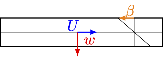
The strain tensor then separates into bending and transverse shear contributions:

\[ \varepsilon_{\alpha\beta}(u) = -z\varepsilon_{\alpha\beta}(\beta), \qquad 2\varepsilon_{\alpha 3}(u) = \partial_\alpha w - \beta_\alpha, \qquad \alpha,\beta\in\{1,2\}. \]

Thus the bending strain is given by \(\varepsilon(\beta)\), while the shear strain is \(\nabla w-\beta\).

8.3. Thickness scaling

Integrating through the thickness gives

\[ \int_{-t/2}^{t/2} z^2\,dz = \frac{t^3}{12}, \qquad \int_{-t/2}^{t/2} 1\,dz = t. \]

Therefore bending scales like \(t^3\), while transverse shear scales like \(t\). After a load rescaling and division by \(t^3\), the weak form of the Reissner-Mindlin problem reads:

Find \((w,\beta)\in H^1_0(\omega)\times [H^1_0(\omega)]^2\) such that

\[ \frac{1}{12}\int_\omega \mathbb{D}\varepsilon(\beta):\varepsilon(\delta)\,dx + \frac{\kappa G}{t^2}\int_\omega (\nabla w-\beta)\cdot(\nabla v-\delta)\,dx = \int_\omega f v\,dx \]

for all \((v,\delta)\in H^1_0(\omega)\times [H^1_0(\omega)]^2\). Here, we denoted the shearing modulus \(G\) and the shear correction factor \(\kappa\) by

\[ G=\frac{E}{2(1+\nu)},\qquad \kappa= \frac56. \]

We note that the shear correction factor \(\kappa\) does not follow from the derivation but is additionally added to compensate for high-order effects of the shear stresses, which are not constant through the thickness.

The factor \(t^{-2}\) is the source of potential shear locking for very thin plates.

8.4. Kirchhoff-Love limit

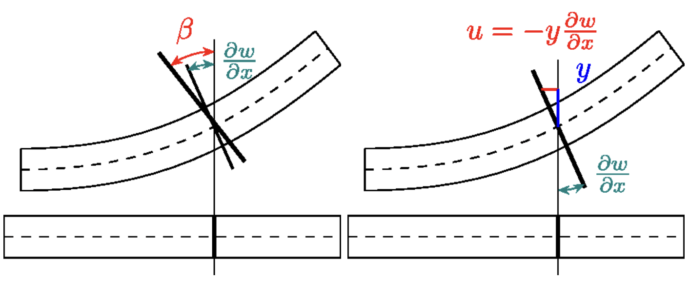
The Kirchhoff-Love assumption says that normals to the midsurface remain normal after deformation. In the linearized setting this eliminates the rotation \(\beta\)

\[ \nabla w - \beta = 0, \qquad \text{hence} \qquad \beta = \nabla w. \]

Inserting this constraint into the bending energy gives the Kirchhoff-Love plate model:

Find \(w\in H^2_0(\omega)\) such that

\[ \int_\omega \mathbb{D}\nabla^2 w : \nabla^2 v\,dx = \int_\omega f v\,dx \qquad \forall v\in H^2_0(\omega). \]

In strong form this is the fourth-order equation

\[ \operatorname{div}\operatorname{div}(\mathbb{D}\nabla^2 w)=f. \]

The Kirchhoff-Love plate model does not suffer from shear locking as the shear has been eliminated. However, the costs we have to pay is that we need to discretize a fourth-order problem, which is more challenging.

8.5. Boundary conditions and physical quantities

For Reissner-Mindlin plates the bending moment and shear force are

\[ M = \frac{1}{12}\mathbb{D}\varepsilon(\beta), \qquad Q = \frac{\kappa G}{t^2}(\nabla w-\beta). \]

Typical boundary conditions for the Reissner-Mindlin plate are given by

boundary conditions	\(w\)	\(\beta_n\)	\(\beta_t\)	resulting conditions
clamped	D	D	D	\(w=0\), \(\beta=0\)
free	N	N	N	\(Q\cdot n=0\), \(Mn=0\)
hard simply supported	D	N	D	\(w=0\), \(n^\top Mn=0\), \(\beta_t=0\)
soft simply supported	D	N	N	\(w=0\), \(Mn=0\)

The boundary conditions for the Kirchhoff-Love plate can be summarized with the bending moment \(M = \mathbb{D}\nabla^2 w\) as

boundary conditions	\(w\)	\(\partial_n w\)	resulting conditions
clamped	D	D	\(w=0\), \(\partial_n w=0\)
simply supported	D	N	\(w=0\), \(M_{nn}=0\)
free	N	N	\(M_{nn}=0\), \(\frac{\partial M_{nt}}{\partial t}+\mathrm{div}(M)\cdot n=0\)
free (corner condition)			\([\![ M_{nt}]\!]_x = M_{n_1t_1}(x)-M_{n_2t_2}(x)=0\quad \forall x\in \mathcal{V}_{\Gamma_f}\)

\(\mathcal{V}_{\Gamma_f}\) denotes the set of corner points where the two adjacent edges belong to \(\Gamma_f\). Here, \(n\) and \(t\) denote the outer normal and tangential vector on the plate boundary. Physically, \(M_{nn}:=n^\top M n\) is the normal bending moment, \(\partial_t(t^\top M n) + n^\top\mathrm{div}(M)\) the effective transverse shear force, and \(\sigma_{nt}:=t^\top M n\) the torsion moment. Further, the effective shear force \(Q_{\mathrm{eff}}\) is given by \(Q_{\mathrm{eff}}=-\mathrm{div}(M)\).

The mixed methods in the next two notebooks are designed around the physical variables rotations and moments.