Heavy top without kinematik constraints

12.6. Heavy top without kinematik constraints#

example from

Evaluation and implementation of Lie group integration methods for rigid multibody systems

S. Holzinger, M. Arnold, J. Gerstmayr

Section 4.1

https://link.springer.com/article/10.1007/s11044-024-09970-8

import ngsolve

from ngsolve import *
from netgen.occ import *
import ipywidgets as widgets
from ngsolve.comp import GlobalSpace
from ngsolve.webgui import Draw
from ngsolve.solvers import Newton
from ngsolve.comp import DifferentialSymbol
# ngsglobals.msg_level=10

mass = 15
Jxx = Jzz = 0.234375
Jyy = 0.468750  # (= 2*Jxx, so its a disk)
omega0 = CF( (0,150,-4.61538) )

b = sqrt(3/2 * Jyy/mass)
rho = mass/(4*b*b)     # kg/ m**2
b, rho

(0.21650635094610965, 80.00000000000001)

center = Pnt( (0,1,0) )
disk = WorkPlane(Axes((0,1,0), Y)).RectangleC(2*b, 2*b).Face()
shape = Glue ([disk, Segment( (0,0,0), (0,1,0)) ])
shape.vertices.Min(Y).name="A"
mesh = Mesh(OCCGeometry(shape).GenerateMesh(maxh=3))
Draw (mesh);

RBshapes = CF ( ( 1, 0, 0,
                  0, 1, 0,
                  0, 0, 1,
                  y, -x, 0,
                  0, z, -y,
                  -z, 0, x) ).Reshape((6,3)).Compile() # realcompile=True, wait=True)
RBspace = GlobalSpace (mesh, order=1, basis = RBshapes)

SYMshapes = CF ( ( 1, 0, 0, 0, 0, 0, 0, 0, 0,
                   0, 0, 0, 0, 1, 0, 0, 0, 0,
                   0, 0, 0, 0, 0, 0, 0, 0, 1,
                   0, 1, 0, 1, 0, 0, 0, 0, 0,
                   0, 0, 1, 0, 0, 0, 1, 0, 0,
                   0, 0, 0, 0, 0, 1, 0, 1, 0) ).Reshape((6,9)).Compile() # realcompile=True, wait=True)
SYMspace = GlobalSpace (mesh, order=1, basis = SYMshapes)

P1shapes = CF ( ( 1, 0, 0,
                  0, 1, 0,
                  0, 0, 1,
                  x, 0, 0,
                  0, x, 0,
                  0, 0, x,
                  y, 0, 0,
                  0, y, 0,
                  0, 0, y,
                  z, 0, 0,
                  0, z, 0,
                  0, 0, z)).Reshape((12,3)).Compile() # realcompile=True, wait=True)
P1space = GlobalSpace (mesh, order=1, basis = P1shapes)
P1space.AddOperator("dx", VOL, P1shapes.Diff(x))
P1space.AddOperator("dy", VOL, P1shapes.Diff(y))
P1space.AddOperator("dz", VOL, P1shapes.Diff(z))

def MyGrad(gf):
    return CF( (gf.Operator("dx"), gf.Operator("dy"), gf.Operator("dz") )).Reshape((3,3)).trans
def MyGradB(gf):
    return CF( (gf.Operator("dx", BND), gf.Operator("dy", BND), gf.Operator("dz", BND))).Reshape((3,3)).trans
def MyGradBB(gf):
    return CF( (gf.Operator("dx", BBBND), gf.Operator("dy", BBBND), gf.Operator("dz", BBBND))).Reshape((3,3)).trans
              

12.6.1. Livens principle#

[P. Kinon, B. Betsch 23]

\[ \delta S = 0 \quad \text{ with } \quad S(q,v,p) = \int_0^T T(v) - V(q) + \left< p, \dot q - v \right> \, dt \]

with position \(q : [0,T] \rightarrow M\), velocity \(v : [0,T] \rightarrow T_q M\), momentum \(p : [0,T] \rightarrow T^\ast_q M\)

12.6.2. time-stepping#

Rattle algorithm (see Hairer-Lubich-Wanner, page 246)

Variables are

position \(q = a + B x\), an affine linear function, with constraint \(B^T B = I\), i.e. \(B\) is orthogonal (and thus, by continuity, a rotation matrix)
velocity \(v = a + b \wedge x\), in body-frame
momentum \(p = \rho v\)

unknowns in time-step: \(q(t_{n+1}), v(t_{n+1/2}), p(t_{n+1/2}), \hat p := p(t_{n+1}) \)

constraints: \(A(t_{n+1}) = \dot A(t_{n+1}) = (0,0,0)\)

Lagrange parameters: \(f_A(t_n), f_A(t_{n+1})\)

Thesis Linus Knoll

fesR = NumberSpace(mesh)

fes = P1space * RBspace * RBspace * RBspace * fesR**3 * fesR**3
festest = RBspace * RBspace * RBspace * RBspace * SYMspace * fesR**3 * fesR**3

# print ("dimtrial =", fes.ndof, ", dimtest =", festest.ndof)
gfold = GridFunction(fes)
gf = GridFunction(fes)

qold, vold, pold, phatold, fa1old, fa2old = gfold.components
gfq, gfv, gfp, gfphat, gffa1, gffa2 = gf.components

q, v, p, phat, fa1, fa2  = fes.TrialFunction()
dv, dp, du1, du2, dlagsym, da, daprime = festest.TestFunction()

dvert = DifferentialSymbol(BBBND)

tau = 0.0005
P0 = CF( (0, 0, 0) )
PA0 = CF( (0, 1, 0)) 

gfphat.Set ( rho*Cross (omega0, CF((x,y,z))) , definedon=mesh.Boundaries(".*") )

force = CF( (0,0,-9.81*rho) )
dpointA = da
dpointAprime = daprime
qold.Set ( (x, y, z) )

Rnew = MyGrad(q)
Rold = MyGradB(qold)
Rmean = 0.5*(Rold+Rnew)

a = BilinearForm(trialspace=fes, testspace=festest)

# linear part of q is orthogonal:
a += InnerProduct (Rnew.trans*Rnew-Id(3), dlagsym) * ds 

# p = rho*v
a += (rho*v-p)*dv * ds

# dot q = v
# a += (Rmean.trans * (q - qold) - tau*v) * dp  * ds
# a +=  ( 1/2*(qold-q + tau * Rold*v)*(Rold*dp) + 1/2*(qold-q+tau*Rnew*v) * (Rnew*dp) ) * ds
a += (qold + tau/2 * Rold*v - (q-tau/2*Rnew*v) ) * (Rmean*dp) * ds     # most accurate

# dot p = f
a += ((Rnew*phat-Rmean*p) - tau/2*force) * (Rnew*du1) * ds
a += ((Rmean*p-Rold*phatold) - tau/2*force) * (Rold*du2) * ds

# forces from Lagrange parameters, in t_n and t_{n+t}:
a += ( (- tau/2*fa1 ) * (Rnew*du1)) *dvert("A")
a += ( (- tau/2*fa2 ) * (MyGradBB(qold)*du2)) *dvert("A")

# constraints and velocity constraints:
a += (q-P0)*dpointA* dvert("A")
a += (phat)*dpointAprime * dvert("A")

# tricky to set initial conditions, since mass matrix alone is singular 
# gfq.Set ( (x, y, z), definedon=mesh.Boundaries(".*")  )
qs,dqs = P1space.TnT()
bfset = BilinearForm(qs*dqs*ds + qs.Operator("dy")*dqs.Operator("dy")*ds).Assemble()
lfset = LinearForm(CF((x,y,z))*dqs*ds + CF((0,1,0))*dqs.Operator("dy")*ds).Assemble()
gfq.vec[:] = bfset.mat.Inverse()*lfset.vec

scene = Draw (gf.components[1], mesh, deformation=(gf.components[0]-CF((x,y,z))), center=(0,0,0), radius=1.2)

tw = widgets.Text(value='t = 0')
display(tw)

t = 0
tt = []
Epott = []
Ekint = []
Et = []
axt, ayt, azt = [], [], []
# with TaskManager(): # pajetrace=10**9):
while t < 1-1e-10:
    gfold.vec[:] = gf.vec
    Newton(a=a, u=gf, printing=False, maxerr=1e-8)
    scene.Redraw()
    t += tau
    tw.value = "t = {t:.2f}".format(t=t)
    Epot = -Integrate (gfq*force*ds, mesh)
    Ekin = Integrate (rho/2*gfv*gfv*ds, mesh)
    tt.append(t)
    Epott.append(Epot)
    Ekint.append(Ekin)
    axt.append (Integrate(gfq[0]*ds, mesh)/(4*b**2))
    ayt.append (Integrate(gfq[1]*ds, mesh)/(4*b**2))
    azt.append (Integrate(gfq[2]*ds, mesh)/(4*b**2))
    Et.append(Epot+Ekin)      

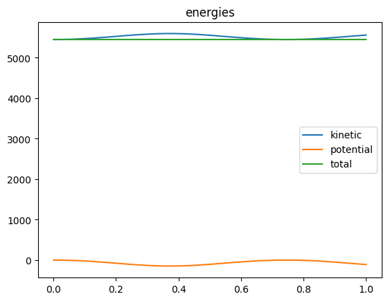
import matplotlib.pyplot as plt
plt.plot (tt, Ekint, label="kinetic")
plt.plot (tt, Epott, label="potential")
plt.plot (tt, Et, label="total")
plt.legend()
plt.title("energies")
plt.show()

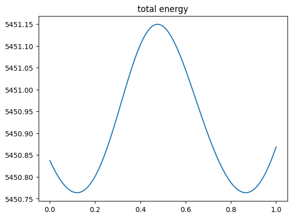
plt.plot (tt, Et)
plt.title("total energy")
plt.show()

plt.plot (tt, axt, label="x")
plt.plot (tt, ayt, label="y")
plt.plot (tt, azt, label="z")
plt.legend()
plt.show()

print (axt[-1], ayt[-1], azt[-1])

../_images/36ed824fd61546130a0cd0767b7fe65ed4ed389ac4aee1dcb4b09320af71ef80.png

../_images/30f961e64c9f1465ad2f5168ee94bf115d8bcec7496cdadf9c6f8385fea8dd79.png

../_images/9071183a8a7fdc78407a406b486fa18d222d38f9ac61abcba6d9dc1c9aa9c0c4.png

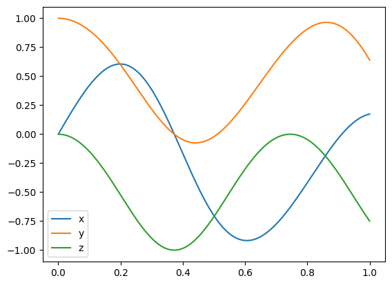
0.1733820676277703 0.639920677477894 -0.7486255306635918

Values at \(t=1\):

\(\tau\)	\(A_x\)	\(A_y\)	\(A_z\)
4e-3	-0.08166	-0.09591	-0.99203
2e-3	0.18651	0.53720	-0.82258
1e-3	0.17802	0.61715	-0.76642
5e-4	0.17458	0.63451	-0.75294
2.5e-4	0.17366	0.63870	-0.74960

with improved velocity integration:

\(\tau\)	\(A_x\)	\(A_y\)	\(A_z\)
4e-3	0.17592	0.62806	-0.75802
2e-3	0.17396	0.63734	-0.75069
1e-3	0.173497	0.639414	-0.749032
5e-4	0.173382	0.639921	-0.748626
2.5e-4	0.173353	0.640047	-0.748524

Heavy top without kinematik constraints

Contents

12.6. Heavy top without kinematik constraints#

12.6.1. Livens principle#

12.6.2. time-stepping#