19.2. Fluid-structure interaction with \(H(\mathrm{div})\)-conforming HDG

In this section we use \(H(\mathrm{div})\)-conforming HDG elements for the Navier-Stokes equations and Lagrangian elements for the elastic wave equation, following [Neunteufel, Schöberl. Fluid-structure interaction with H(div)-conforming finite elements. Computers and Structures, (2021).]. The notation follows the FSI introduction: \(u_f,p_f\) denote the fluid velocity and pressure, \(d_s,u_s\) the solid displacement and velocity, and \(d_m,w_m\) the ALE mesh displacement and velocity.

19.2.1. \(H(\mathrm{div})\)-conforming HDG for Navier-Stokes with upwinding

We quickly recap the \(H(\mathrm{div})\)-conforming HDG method for Navier-Stokes with upwinding for the convection term, as we will need to reformulate it in terms of an ALE formulation; for details see e.g. NGSolve documentation on DG/HDG splitting, [Lehrenfeld, Schöberl. High order exactly divergence-free Hybrid Discontinuous Galerkin Methods for unsteady incompressible flows. Computer Methods in Applied Mechanics and Engineering, (2016).].

To this end, let \(u=(u_T,u_F)\), \(v=(v_T,v_F)\) with \(u_T,v_T\) in the \(H(\mathrm{div})\)-conforming \(BDM^k\) space and \(u_F\), \(v_F\) in the vector-valued tangential facet space \(F_h^k\). We define the tangential jump \([\![ v^\tau]\!] = v_T^\tau-v_F^\tau\) with \(u^\tau= u - (u\cdot n)n\) the tangential projection. Further, \(p\) is in the space of piecewise polynomials \(Q_h^{k-1}\). Then the diffusion, mass, and divergence terms of the Navier-Stokes equations are given by

\[\begin{split} \begin{align*} & A_h^f(u,v)=\sum_{T\in \mathcal{T}^f}\Big(\int_T2\nu\varepsilon(u_T):\varepsilon( v_T)\,dx+\int_{\partial T}\big(-2\nu\varepsilon(u_T)n\cdot[\![ v^\tau]\!]- 2\nu\varepsilon(v_T)n\cdot[\![ u^\tau]\!]+\frac{\nu\alpha k^2}{h}[\![ u^{\tau}]\!]\cdot[\![ v^{\tau}]\!]\big)\,ds\Big),\\ & M^f_h(u,v)=\int_{\Omega_f} u_T\cdot v_T\,dx,\\ & D^f_h(v,p)=-\int_{\Omega_f} p\,\mathrm{div}(v_T)\,dx, \end{align*} \end{split}\]

For the convection we use upwinding

\[ \begin{align*} C^f_h({u},v)= \sum_{T\in\mathcal{T}^f}\Big(-\int_T\nabla v_T{u}_T\cdot{u}_T\,dx+\int_{\partial T} {u}_T\cdot {n}\,{u}^{\mathrm{up}}\cdot v_T\,ds+\int_{\partial T_{\mathrm{out}}} {u}_T\cdot {n}\,({u}_F-{u}_T)^{{\tau}}\cdot v_F\,ds\Big), \end{align*} \]

with the upwind variable \({u}^{\mathrm{up}}\) defined as

\[\begin{split} \begin{align*} & {u}^{\mathrm{up}}= ({u}_T\cdot {n}){n}+\begin{cases} {u}_T^{{\tau}} & \text{ if }{u}\cdot {n} \geq 0\\ {u}_F^{{\tau}} & \text{ if } {u}\cdot {n} < 0 \end{cases}. \end{align*} \end{split}\]

19.2.2. Navier-Stokes in ALE (Arbitrary Lagrangian Eulerian) formulation

Let \(\Phi(\hat x,t)=\hat x+d_m(\hat x,t)\) describe the movement of the fluid mesh, where \(d_m\) is the mesh displacement. For Taylor-Hood elements we used the relation \(u_f\circ\Phi=\hat u_f\), since continuity of \(\hat u_f\) implies continuity of \(u_f\) on the deformed configuration. For a velocity field in \(H(\mathrm{div})\), however, we want to preserve normal continuity and the divergence structure. Therefore, we use the Piola transformation

\[ \begin{align*} u_f\circ\Phi =P_{\Phi}[\hat{u}_f]= \frac{1}{J_m} F_m \hat{u}_f, \qquad F_m=\nabla \Phi,\quad J_m=\det(F_m). \end{align*} \]

As a result the chain rule now reads

\[ \begin{align*} \nabla_xu_f\circ\Phi = \nabla_{\hat{x}} (P_{\Phi}[\hat{u}_f])F_m^{-1}. \end{align*} \]

The Piola transformation also depends on the time. Thus we obtain additional terms from the chain rule of the time derivative

\[ \begin{align*} \frac{\partial u_f}{\partial t}\circ\Phi = \frac{1}{J_m}(\nabla_{\hat{x}}w_m-\mathrm{tr}(\nabla_{\hat{x}}w_mF_m^{-1})F_m)\hat{u}_f +P_{\Phi}\left[\frac{\partial \hat{u}_f}{\partial t}\right] - \nabla_{\hat{x}} P_{\Phi}[\hat{u}_f]F_m^{-1}w_m. \end{align*} \]

To avoid implementing all chain rules involving deformation gradients and Jacobian determinants by hand, see [Neunteufel, Schöberl. Fluid-structure interaction with H(div)-conforming finite elements. Computers and Structures, (2021).] for details, we use the dx(deformation=mesh_deformation) flag. Then NGSolve evaluates integrals on the deformed configuration. Only the additional terms from the time derivative of the Piola transformation have to be added explicitly.

19.2.3. Interface conditions

For \(H(\mathrm{div})\)-conforming HDG, the fluid velocity has an element field \(u_T^f\) and a tangential facet field \(u_F^f\). The solid velocity \(u_s\) is represented by Lagrangian elements. We therefore enforce velocity continuity at the interface with Lagrange multipliers: one multiplier for the normal component and one for the tangential component. The mesh displacement is still represented by one global Lagrange space and satisfies \(d_m=d_s\) on the interface.

\[\begin{split} \begin{align*} &\int_{\Gamma_I} ({u}_T^f-u_s)^{n}\,\lambda_n\,ds+\int_{\Gamma_I} (v_T^{f}-v_s)^{n}\,{\mu}_n\,ds=0,\\ &\int_{\Gamma_I}({u}_F^f-u_s)^{t}\,\lambda_t\,ds +\int_{\Gamma_I} (v_F^{f}-v_s)^{t}\,\mu_t\, ds =0, \end{align*} \end{split}\]

and these interface terms are evaluated on the deformed interface in the ALE setting.

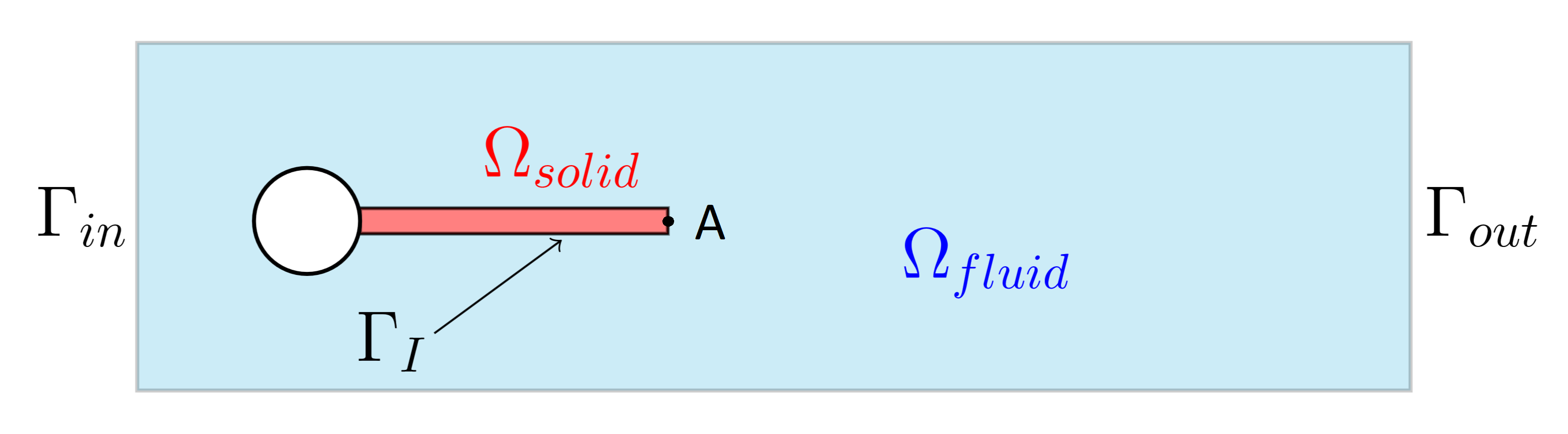
19.2.4. Benchmark example

We will consider the following benchmark proposed in [Turek, Hron. Proposal for numerical benchmarking of fluid-structure interaction between an elastic object and laminar incompressible flow. In: Fluid-Structure Interaction: Modelling, Simulation, Optimisation, 2006]. It is based on the classical flow around cylinder benchmark [Schäfer, Turek, Durst, Krause, Rannacher. Benchmark computations of laminar flow around a cylinder. In: Flow simulation with high-performance computers II, 1996], where additionally an elastic flag is “glued” behind the obstacle.

We choose the space-dependent function \(h(x)\) in the deformation extension problem to be large close to the elastic solid’s tip and to decrease with the distance.

from ngsolve import *
from netgen.occ import *
from ngsolve.webgui import Draw
import ipywidgets as widgets


tau = 0.004
tend = 2
order = 3

mesh_dirichlet = "wall|outlet|inlet|circ|circ_inner"
fluid_velocity_dirichlet = "wall|inlet|circ|circ_inner"
fluid_facet_dirichlet = "wall|inlet|circ|circ_inner|outlet"
solid_velocity_dirichlet = "circ|circ_inner"
multiplier_dirichlet = "wall|outlet|inlet|circ|circ_inner"
fixed_stokes_boundary = "wall|inlet|circ|interface|circ_inner"

# HDG stabilization parameter
alpha = Parameter(5)

# solid density, Poisson ratio, first Lamé parameter, fluid density,
# dynamic viscosity, and maximal inflow velocity
rho_s, poisson_s, mu_s, rho_f, nu_f, U = 1e4, 0.4, 0.5 * 1e6, 1e3, 1e-3, 1
# second Lamé parameter for solid
lambda_s = 2 * mu_s * poisson_s / (1 - 2 * poisson_s)

# inflow profile
u_inflow = CF((4 * U * 1.5 * y * (0.41 - y) / (0.41 * 0.41), 0))


def GenerateMesh(order, maxh=0.203):
    circle = Circle((0.2, 0.2), r=0.05).Face()
    circle.edges.name = "circ"
    fluid = Rectangle(2.5, 0.41).Face()
    fluid.faces.name = "fluid"
    fluid.edges.Min(X).name = "inlet"
    fluid.edges.Max(X).name = "outlet"
    fluid.edges.Min(Y).name = "wall"
    fluid.edges.Max(Y).name = "wall"
    solid = (
        MoveTo(0.248989794855664, 0.19).Rectangle(0.6 - 0.248989794855664, 0.02).Face()
    )
    solid.faces.name = "solid"
    solid.edges.name = "interface"

    domain_fluid = (fluid - circle) - solid
    solid.edges["circ"].name = "circ_inner"
    solid.edges.Min(X).name = "circ_inner"
    domain = Glue([domain_fluid, solid])

    mesh = Mesh(OCCGeometry(domain, dim=2).GenerateMesh(maxh=maxh))
    mesh.Curve(order)

    return mesh


mesh = GenerateMesh(order=order)
Draw(mesh);

For the spatial discretization we use an \(H(\mathrm{div})\) element field, a tangential facet field, and an \(L^2\) pressure for the fluid. The solid velocity and the mesh displacement are represented by \(H^1\)-conforming spaces. The Lagrange multiplier space lives on the interface and couples the HDG fluid velocity to the solid velocity.

V1 = VectorH1(mesh, order=order, dirichlet=mesh_dirichlet)
V2 = HDiv(
    mesh,
    order=order,
    dirichlet=fluid_velocity_dirichlet,
    definedon="fluid",
    hodivfree=True,
)
V3 = TangentialFacetFESpace(
    mesh, order=order, dirichlet=fluid_facet_dirichlet, definedon="fluid"
)
V4 = VectorH1(mesh, order=order, dirichlet=solid_velocity_dirichlet, definedon="solid")
Q = L2(mesh, order=0, definedon="fluid", lowest_order_wb=True)
# Lagrange multiplier forcing continuity of velocities across the interface
V5 = SurfaceL2(mesh, order=order, dirichlet=multiplier_dirichlet) ** 2

X = V2 * V3 * Q * V1 * V4 * V5
Y = V2 * V3 * Q

(u, uhat, p, d, v, f), (ut, uhatt, pt, dt, vt, ft) = X.TnT()

gf_solution = GridFunction(X)
gf_solution_old = GridFunction(X)

fluid_velocity, fluid_facet_velocity, pressure, mesh_deformation, solid_velocity, multiplier = gf_solution.components
fluid_velocity_old, fluid_facet_velocity_old, pressure_old, mesh_deformation_old, solid_velocity_old, multiplier_old = gf_solution_old.components

I = Id(mesh.dim)
F = Grad(d) + I
C = F.trans * F
Fold = Grad(mesh_deformation_old) + I
Cold = Fold.trans * Fold


n, h = specialcf.normal(2), specialcf.mesh_size


def tang(vec):
    return vec - (vec * n) * n


def norma(vec):
    return (vec * n) * n


def Stress(mat):
    return mu_s * mat + lambda_s / 2 * Trace(mat) * I

For the time discretization we will use the Crank-Nicolson method

\[\begin{align*} \int_{t^n}^{t^{n+1}} f(s)\,ds \approx \frac{\tau}{2}(f(t^{n+1})+f(t^n)). \end{align*}\]

Only the pressure constraint is handled with implicit Euler.

# For Stokes problem
stokes = BilinearForm(Y, symmetric=True, check_unused=False)
stokes += (
    nu_f * rho_f * InnerProduct(2 * Sym(Grad(u)), Sym(Grad(ut)))
    - div(u) * pt
    - div(ut) * p
    - 1e-8 * p * pt
) * dx("fluid")
stokes += (
    nu_f
    * rho_f
    * (
        InnerProduct(2 * Sym(Grad(u)) * n, tang(uhatt - ut))
        + InnerProduct(2 * Sym(Grad(ut)) * n, tang(uhat - u))
        + alpha * order * order / h * InnerProduct(tang(uhatt - ut), tang(uhat - u))
    )
) * dx("fluid", element_boundary=True)
stokes.Assemble()

compile_integrands = False

######################################### SOLID #############################################
bfa = BilinearForm(X, symmetric=False, check_unused=False, condense=True)
bfa += (
    (1 / tau * (d - mesh_deformation_old) - 0.5 * (v + solid_velocity_old)) * dt
    + rho_s / tau * (v - solid_velocity_old) * vt
    + 2 * InnerProduct(F * Stress(0.5 * (0.5 * (C + Cold) - I)), Grad(vt))
).Compile(compile_integrands, wait=True) * dx("solid")


def minCF(a, b):
    return IfPos(a - b, b, a)


gf_dist = GridFunction(H1(mesh, order=2))
gf_dist.Set(minCF((x - 0.6) ** 2 + (y - 0.19) ** 2, (x - 0.6) ** 2 + (y - 0.21) ** 2))


def NeoHookExt(C, mu=1, lam=1):
    return 0.5 * mu * (Trace(C - I) + 2 * mu / lam * Det(C) ** (-lam / 2 / mu) - 1)


bfa += Variation(
    1e-20 * mu_s / sqrt(gf_dist * gf_dist + 1e-12) * NeoHookExt(C) * dx("fluid")
).Compile(compile_integrands, wait=True)

################################# FLUID ##############################################
grad_mesh_velocity = (Grad(d) - Grad(mesh_deformation_old)) / tau
mesh_velocity = (d - mesh_deformation_old) / tau
relative_velocity = u - mesh_velocity
relative_normal_velocity = relative_velocity * n
upwind = (u * n) * n + IfPos(relative_normal_velocity, tang(u), tang(uhat))

cfinner = (
    nu_f * rho_f * InnerProduct(Sym(Grad(u)) + Sym(Grad(fluid_velocity_old)), Sym(Grad(ut)))
    - div(u) * pt
    - div(ut) * p
    - rho_f * InnerProduct(0.5 * (u + fluid_velocity_old), Grad(ut) * relative_velocity)
    + rho_f * InnerProduct(0.5 * grad_mesh_velocity * (u + fluid_velocity_old), ut)
    + rho_f / tau * (u - fluid_velocity_old) * ut
)
facet_jump_midpoint = 0.5 * tang(uhat - u + fluid_facet_velocity_old - fluid_velocity_old)

cfouter = nu_f * rho_f * (
    InnerProduct(Sym(Grad(u) + Grad(fluid_velocity_old)) * n, tang(uhatt - ut))
    + InnerProduct(2 * Sym(Grad(ut)) * n, facet_jump_midpoint)
    + alpha
    * order
    * order
    / h
    * InnerProduct(tang(uhatt - ut), facet_jump_midpoint)
) + rho_f * (
    relative_normal_velocity * upwind * ut
    + IfPos(relative_normal_velocity, 1, 0) * relative_normal_velocity * facet_jump_midpoint * uhatt
)
bfa += cfinner.Compile(compile_integrands, wait=True) * dx("fluid", deformation=mesh_deformation)
bfa += cfouter.Compile(compile_integrands, wait=True) * dx(
    "fluid", element_boundary=True, deformation=mesh_deformation
)
# interface
bfa += (
    (norma(v - u.Trace()) + tang(v - uhat.Trace())) * ft
    + (norma(vt - ut.Trace()) + tang(vt - uhatt.Trace())) * f
).Compile(compile_integrands, wait=True) * ds("interface", deformation=mesh_deformation)

proxy not matching space, checking if it is working anyway

To increase the inflow velocity depending on time, we have to extend the new velocity into the domain before solving the system. This can be done by solving a Stokes problem with the new velocity as Dirichlet data only on the fluid domain. To tell the solver on which domain it should work, we have to define the corresponding degrees of freedom, which is done in terms of bitarrays.

bt_stokes = Y.FreeDofs() & ~Y.GetDofs(mesh.Materials("solid"))
bt_stokes &= ~Y.GetDofs(mesh.Boundaries(fixed_stokes_boundary))
inv_stokes = stokes.mat.Inverse(bt_stokes, inverse="")

gf_stokes = GridFunction(Y)
stokes_velocity, stokes_facet_velocity, stokes_pressure = gf_stokes.components
res_stokes = gf_stokes.vec.CreateVector()
stokes_velocity.Set(u_inflow, BND, definedon=mesh.Boundaries("inlet"))
res_stokes.data = stokes.mat * gf_stokes.vec
gf_stokes.vec.data -= inv_stokes * res_stokes
fluid_velocity.vec.data = stokes_velocity.vec
fluid_facet_velocity.vec.data = stokes_facet_velocity.vec
pressure.vec.data = stokes_pressure.vec

scene_u = Draw(
    fluid_velocity,
    mesh.Materials("fluid"),
    "velocity",
    deformation=mesh_deformation,
    order=3,
    max=2,
)
scene_p = Draw(pressure, mesh.Materials("fluid"), "pressure", deformation=mesh_deformation)
scene_d = Draw(mesh_deformation, mesh, "deformation")

gf_history = GridFunction(X, multidim=0)

w = gf_solution.vec.CreateVector()
res = gf_solution.vec.CreateVector()

Time loop.

# Calculate quantities of interest
def CalcForces(disp_x, disp_y):
    dmidx, dmidy = mesh_deformation(0.6, 0.2)
    disp_x.append(dmidx)
    disp_y.append(dmidy)
    return


disp_x = [0]
disp_y = [0]
times = [0]

t = 0
i = 0

tw = widgets.Text(value="t = 0")
display(tw)

with TaskManager():
    while t < tend - tau / 2.0:
        t += tau

        gf_solution_old.vec.data = gf_solution.vec

        # Newton
        for step in range(2):
            bfa.AssembleLinearization(gf_solution.vec)
            inv = bfa.mat.Inverse(bfa.space.FreeDofs(bfa.condense), inverse="")
            bfa.Apply(gf_solution.vec, res)

            if bfa.condense:
                res.data += bfa.harmonic_extension_trans * res
            w.data = inv * res
            if bfa.condense:
                w.data += bfa.harmonic_extension * w
                w.data += bfa.inner_solve * res

            gf_solution.vec.data -= w

        if i % 4 == 0:
            scene_u.Redraw()
            scene_p.Redraw()
            scene_d.Redraw()

        if i % 20 == 0:
            gf_history.AddMultiDimComponent(gf_solution.vec)

        times.append(t)
        CalcForces(disp_x, disp_y)
        i += 1
        tw.value = f"t = {round(t,5)}"

Draw(
    gf_history.components[0],
    mesh.Materials("fluid"),
    animate=True,
    min=0,
    max=2,
    autoscale=True,
    deformation=gf_history.components[3],
    order=3,
);

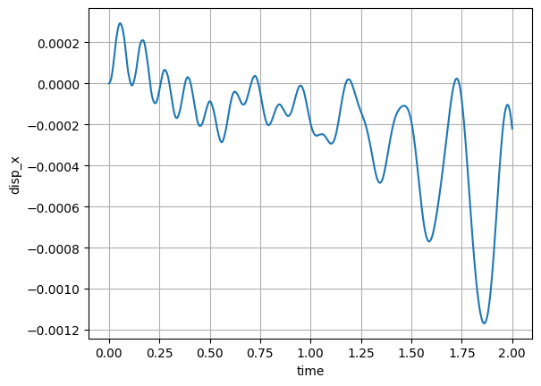
Draw results over time. They become periodic after some time.

import matplotlib.pyplot as plt

plt.plot(times, disp_x)
plt.xlabel("time")
plt.ylabel("disp_x")
plt.grid(True)
plt.show()

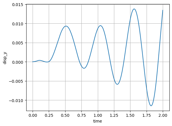
plt.plot(times, disp_y)
plt.xlabel("time")
plt.ylabel("disp_y")
plt.grid(True)
plt.show()