11. Linear shells

Shells are thin three-dimensional structures whose mechanical behavior is governed by a curved midsurface and a small thickness. Shells are the “primadonna of structures” (Ramm, 1986). On the one hand, if properly designed, they can exhibit an optimal ratio of stiffness to weight. On the other hand, especially for thin shells, they can be extremely sensitive to imperfections and develope unstable behavior.

For a comprehensive introduction and derivation to shell models we refer to the literature, e.g.

• Chapelle, Bathe., The finite element analysis of shells - fundamentals. 2011,

• Bischoff, Ramm, Irslinger. Models and Finite Elements for Thin-Walled Structures. 2017,

• Ciarlet. An Introduction to Differential Geometry with Applications to Elasticity. 2005,

• Ciarlet. Mathematical modelling of linearly elastic shells. 2001.

11.1. From a thin body to a midsurface

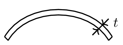
A shell is described by a midsurface \(\mathcal{S}\subset\mathbb{R}^3\) and a thickness \(t\). Points in the thin three-dimensional body are approximated by

\[ x = \xi + z\hat\nu(\xi), \qquad \xi\in\mathcal{S},\quad z\in[-t/2,t/2], \]

where \(\hat\nu\) is the unit normal of the reference midsurface.

The shell unknown is the midsurface displacement

\[ u:\mathcal{S}\to\mathbb{R}^3. \]

For Kirchhoff-Love shells the normal director is not an independent unknown: normals remain normal to the deformed midsurface. Thus the model has no transverse shear energy.

11.2. Shell energies

energy	scaling	meaning
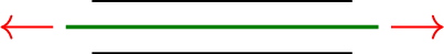
membrane	\(t\)	stretching of the midsurface
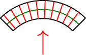
bending	\(t^3\)	change of curvature / normal field
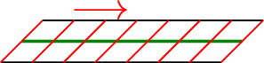
shear	\(t\)	director not perpendicular to midsurface

In this first shell notebook we focus on the linear Kirchhoff-Love case: membrane plus bending, but no shear. Reissner-Mindlin shells add shear and will be a natural transition to TDNNS later.

membrane	bending	shear

11.3. Linear Kirchhoff-Love shell

A compact linear Kirchhoff-Love shell energy is

\[ \mathcal{W}_{\rm KL}(u) =\int_{\mathcal{S}}\left( \frac{t}{2}\|\varepsilon_{\mathcal{S}}(u)\|_{\mathbb{C}}^2 +\frac{t^3}{24}\|\mathcal{H}_{\hat\nu}(u)\|_{\mathbb{C}}^2 \right)\,ds -\int_{\mathcal{S}}f\cdot u\,ds. \]

Here \(\varepsilon_{\mathcal{S}}(u)=\operatorname{sym}(\nabla_{\mathcal{S}}^{\rm cov}u)\) is the linearized membrane strain, i.e. the tangential-tangential part of the symmetric surface gradient. The bending strain is the normal curvature variation

\[ \mathcal{H}_{\hat\nu}(u) = \sum_{i=1}^3 \nabla_{\mathcal{S}}^2 u_i\,\hat\nu_i. \]

For a flat plate, the membrane and bending parts decouple. For a curved shell they are coupled by the geometry of \(\mathcal{S}\).

11.4. Hellan-Herrmann-Johnson (HHJ) for linear Kirchhoff-Love shells

For Kirchhoff-Love plates the HHJ method avoids globally \(H^2\)-conforming spaces by introducing the bending moment

\[ \sigma = \mathbb{D}\nabla^2 w. \]

For a Kirchhoff-Love shell we use the same idea, but the scalar plate Hessian is replaced by the normal curvature variation \(\mathcal{H}_{\hat\nu}(u)\):

\[ \sigma = \mathbb{C}\mathcal{H}_{\hat\nu}(u). \]

The curved-surface HHJ pairing is the analogue of the plate pairing. The facet unknown stores the normal derivative trace, and the moment tensor lives in a surface \(H(\operatorname{div}\operatorname{div})\) space. The HHJ shell pairing is the curved-surface analogue of the plate pairing:

\[ \langle \sigma,\mathcal{H}_{\hat\nu}(u)\rangle = \sum_{T}\int_T \sigma:\mathcal{H}_{\hat\nu}(u)\,ds - \sum_E\int_E [\![(\nabla_{\mathcal{S}}u)_{\mu\nu}]\!]\sigma_{\mu\mu}\,dl. \]

For a flat plate this reduces to the familiar term involving \([\![\partial_n w]\!]\sigma_{nn}\), see [Neunteufel, Schöberl. The Hellan-Herrmann-Johnson and TDNNS methods for linear and nonlinear shells. Computers & Structures, 305 (2024).].

11.5. Membrane locking and Regge interpolation

For thin shells in bending-dominated regimes, the membrane energy imposes an almost-inextensional constraint. Standard displacement spaces often cannot represent this constraint well, so the displacement collapses towards zero. This is called membrane locking.

The cure used here is to weaken the membrane strain by interpolation into a lower-order Regge space following [Neunteufel, Schöberl. Avoiding membrane locking with Regge interpolation. Comput. Methods Appl. Mech. Eng. 373, (2021)]:

\[ \operatorname{sym}(\nabla_{\mathcal{S}}^{\rm cov}u) \quad\longrightarrow\quad \mathcal{I}^{\rm Reg}\operatorname{sym}(\nabla_{\mathcal{S}}^{\rm cov}u). \]

The Regge space is tangential-tangential continuous, matching the geometric nature of metric strains.

11.6. Sydney Opera House

The following example uses a simple geometric model inspired by the Sydney Opera House (thanks Sebastian Hirnschall).

from ngsolve import *
from netgen.occ import *
from ngsolve.webgui import Draw

# first panel
v1l = Pnt(0, -10, 0.1)
v1t = Pnt(-6, 0, 10.5)
w1 = Wire(ArcOfCircle(v1l, Vec(-0.3, 0.4, 1), v1t))

v12l = Pnt(0.25, -10, 0.1)
v12t = Pnt(-0.5, 0, 11)
w12 = Wire(ArcOfCircle(v12l, Vec(-0.25, 0.3, 1), v12t))

v2l = Pnt(0.5, -10, 0.1)
v2t = Pnt(5 - 0.15, 0, 10)
w2 = Wire(ArcOfCircle(v2l, Vec(0, 0.2, 1), v2t))

# vent
v1lv = Pnt(1, -10.5, 1.5)
v1tv = Pnt(5, 0, 10)
w2v = Wire(ArcOfCircle(v1lv, Vec(0, 0.4, 1), v1tv))

v2lv = Pnt(4.5, -10.5, 0.5)
v2tv = v1tv
w3v = Wire(ArcOfCircle(v2lv, Vec(0, 0.2, 1), v2tv))

v3l = Pnt(5, -10, 1)
v3t = Pnt(5 + 0.15, 0, 10)
w3 = Wire(ArcOfCircle(v3l, Vec(0, 0, 1), v3t))

v4l = Pnt(5.5, -10 - 1, 1)
v4t = Pnt(3.5, 0, 15)
w4 = Wire(ArcOfCircle(v4l, Vec(0, 0, 1), v4t))

# second panel
v212l = Pnt(5.5 + 0.25, -10 - 1, 1)
v212t = Pnt(3.5 + 5.5, 0, 11 + 2)
w212 = Wire(ArcOfCircle(v212l, Vec(0, 0, 1), v212t))

v22l = Pnt(5.5 + 0.5, -10 - 1, 1)
v22t = Pnt(3.5 + 11 - 0.15, 0, 10 + 1)
w22 = Wire(ArcOfCircle(v22l, Vec(0.2, 0, 1), v22t))

# vent
v21lv = Pnt(5.5 + 0.5 + 0.5, -10 - 1.5, 1.5)
v21tv = Pnt(3.5 + 11, 0, 10 + 1)
w22v = Wire(ArcOfCircle(v21lv, Vec(0.3, 0.1, 1), v21tv))

v22lv = Pnt(3.5 + 11 - 1.5, -10 - 1.5, 1)
v22tv = v21tv
w23v = Wire(ArcOfCircle(v22lv, Vec(-0.2, 0, 1), v22tv))

v23l = Pnt(3.5 + 11, -10 - 1, 0)
v23t = Pnt(3.5 + 11 + 0.15, 0, 10 + 1)
w23 = Wire(ArcOfCircle(v23l, Vec(0, 0, 1), v23t))

v24l = Pnt(3.5 + 11, -10 - 1.5, 0)
v24t = Pnt(11, 0, 14 + 8)
w24 = Wire(ArcOfCircle(v24l, Vec(-0.1, 0, 1), v24t))

# third panel
v312l = Pnt(3.5 + 11 + 0.25, -10 - 1.5, 0)
v312t = Pnt(11 + 9, 0, 11 + 6.5)
w312 = Wire(ArcOfCircle(v312l, Vec(0.2, 0, 1), v312t))

v32l = Pnt(3.5 + 11 + 0.5, -10 - 1.5, 0)
v32t = Pnt(11 + 15 - 0.25, 0, 9)
w32 = Wire(ArcOfCircle(v32l, Vec(1, 0, 1), v32t))

# fourth panel vent
v32lv = Pnt(3.5 + 11 + 0.5 + 4, -10 - 1.5 - 0.5, 3)
v32tv = Pnt(11 + 15 - 0.25, 0, 9)
w32v = Wire(ArcOfCircle(v32lv, Vec(0.6, 0.3, 1), v32tv))

v33lv = Pnt(3.5 + 11 + 0.5 + 9, -10 - 1.5 - 0.5, 2)
v33tv = Pnt(11 + 15, 0, 9)
w33v = Wire(ArcOfCircle(v33lv, Vec(0, 0.3, 1), v33tv))

v34lv = Pnt(3.5 + 11 + 17 - 2, -10 - 1.5 - 0.5, 3)
v34tv = Pnt(11 + 15, 0, 9)
w34v = Wire(ArcOfCircle(v34lv, Vec(-0.6, 0.3, 1), v34tv))

v41l = Pnt(3.5 + 11 + 17, -10 - 1.5, 0)
v41t = Pnt(11 + 15 + 0.25, 0, 9)
w41 = Wire(ArcOfCircle(v41l, Vec(-0.5, 0, 1), v41t))

v42l = Pnt(3.5 + 11 + 17 + 0.25, -10 - 1.5, 0)
v42t = Pnt(3.5 + 11 + 17 + 0.25 - 0.5, 0, 11.75)
w42 = Wire(ArcOfCircle(v42l, Vec(0, 0, 1), v42t))

v43l = Pnt(3.5 + 11 + 17 + 0.5, -10 - 1.5, 0)
v43t = Pnt(3.5 + 11 + 17 + 0.5 + 5, 0, 12)
w43 = Wire(ArcOfCircle(v43l, Vec(0.25, 0, 1), v43t))

shape = Glue(
    [w1, w12, w2, w2v, w3v, w3, w4]
    + [w212, w22, w22v, w23v, w23, w24]
    + [w312, w32, w32v, w33v, w34v]
    + [w41, w42, w43]
)
Draw(shape);

f1 = ThruSections([w2, w12, w1], solid=False)
f2 = ThruSections([w2v, w2], solid=False)
v1 = ThruSections([w3v, w2v], solid=False)
v2 = ThruSections([w3, w3v], solid=False)
f3 = ThruSections([w4, w3], solid=False)

f4 = ThruSections([w22, w212, w4], solid=False)
f5 = ThruSections([w22v, w22], solid=False)
v3 = ThruSections([w23v, w22v], solid=False)
v4 = ThruSections([w23, w23v], solid=False)
f6 = ThruSections([w24, w23], solid=False)

f7 = ThruSections([w32, w312, w24], solid=False)
v5 = ThruSections([w32v, w32], solid=False)
v6 = ThruSections([w33v, w32v], solid=False)
v7 = ThruSections([w34v, w33v], solid=False)

f8 = ThruSections([w41, w34v], solid=False)
f9 = ThruSections([w43, w42, w41], solid=False)
shell = Glue([f1, f2, f3, f4, f5, f6, f7, f8, f9, v1, v2, v3, v4, v5, v6, v7])

shell = Glue([shell, shell.Mirror(Axes((0, 0, 0), Y))])
shell.edges[Z <= 0.2].name = "fix"

shell.vertices.hpref = 1
shell.edges.hpref = 1
shell.faces.col = (222 / 255, 224 / 255, 204 / 255, 1)

Draw(shell)
print("model created by Sebastian Hirnschall")

model created by Sebastian Hirnschall

mesh = Mesh(OCCGeometry(shell).GenerateMesh(maxh=2))
mesh.RefineHP(1)
mesh.Curve(3)
Draw(mesh);

The code below is the shell analogue of the hybridized HHJ plate formulation. The displacement is vector-valued, the moment tensor is a surface \(H(\operatorname{div}\operatorname{div})\) field, and a normal-facet variable represents the normal derivative trace.

thickness = 0.1
order = 4

young_modulus = 2.85e4
poisson = 0.3


def MaterialNorm(mat, young_modulus, poisson):
    return young_modulus / (1 - poisson**2) * (
        (1 - poisson) * InnerProduct(mat, mat) + poisson * Trace(mat) ** 2
    )


def MaterialNormInv(mat, young_modulus, poisson):
    return (1 + poisson) / young_modulus * (
        InnerProduct(mat, mat) - poisson / (poisson + 1) * Trace(mat) ** 2
    )

fes_u = VectorH1(mesh, order=order, dirichlet_bbnd="fix")
fes_sigma = HDivDivSurface(mesh, order=order - 1, discontinuous=True)
fes_normal_trace = NormalFacetSurface(mesh, order=order - 1)

fes = fes_u * fes_sigma * fes_normal_trace
(u, sigma, normal_trace) = fes.TrialFunction()
sigma, normal_trace = sigma.Trace(), normal_trace.Trace()

fes_regge = HCurlCurl(mesh, order=order - 1)

normal = specialcf.normal(3)
tangent = specialcf.tangential(3)
conormal = Cross(normal, tangent)

Ptau = Id(3) - OuterProduct(normal, normal)
grad_u = Grad(u).Trace()

# Linearized membrane strain: tangential-tangential symmetric surface gradient.
eps_membrane = 0.5 * (Ptau * grad_u + grad_u.trans * Ptau)

# Normal curvature variation, the shell analogue of the plate Hessian.
normal_hessian = (u.Operator("hesseboundary").trans * normal).Reshape((3, 3))

bfa = BilinearForm(fes, symmetric=True, condense=True)

# Membrane part. The Regge interpolation weakens membrane locking.
bfa += Variation(
    thickness
    / 2
    * MaterialNorm(Interpolate(eps_membrane, fes_regge), young_modulus, poisson)
    * ds
)

# Bending part in HHJ form.
bfa += Variation(
    -12
    / thickness**3
    / 2
    * MaterialNormInv(sigma, young_modulus, poisson)
    * ds
)
bfa += Variation(InnerProduct(sigma, normal_hessian) * ds)
bfa += Variation(
    sigma[conormal, conormal]
    * (normal_trace - grad_u[normal, :])
    * conormal
    * ds(element_boundary=True)
)

force = CF((0, 0, -0.01))
bfa += Variation(-force * u * ds)

gf_solution = GridFunction(fes)

with TaskManager():
    solvers.Newton(a=bfa, u=gf_solution, maxerr=1e-8, printing=False)

gf_u, gf_sigma, gf_normal_trace = gf_solution.components

Draw(gf_u, scale=10, deformation=True);

Draw(Norm(gf_sigma), mesh, order=3, max=0.2);

11.7. What comes next

• Reissner-Mindlin shells add a shear term and an independent director/shear variable.

• The TDNNS viewpoint is the natural continuation of Reissner-Mindlin plates.

• Nonlinear Koiter and Naghdi shells reuse the same membrane, bending, and shear energies, but the strain measures are no longer linearized.