9. Reissner-Mindlin plates with TDNNS

This notebook discusses shear locking for Reissner-Mindlin plates and shows how the TDNNS method can be used to avoid it. The important point is the discrete Kirchhoff constraint: for small thickness, the method must be able to fulfill the constraint

\[ \beta = \nabla w \]

sufficiently well in the discrete setting.

9.1. Reissner-Mindlin energy

With the vertical deflection \(w\) and rotation \(\beta\), the Reissner-Mindlin energy reads

\[ \mathcal{W}_{\rm RM}(w,\beta) = \frac12\int_\Omega \mathbb{D}\varepsilon(\beta):\varepsilon(\beta)\,dx + \frac12\frac{\kappa G}{t^2}\int_\Omega |\nabla w-\beta|^2\,dx - \int_\Omega f w\,dx. \]

The weak formulation is: Find \((w,\beta)\in H^1_0(\Omega)\times [H^1_0(\Omega)]^2\) such that for all \((v,\delta)\in H^1_0(\Omega)\times [H^1_0(\Omega)]^2\)

\[ \frac{1}{12}\int_\Omega \mathbb{D}\varepsilon(\beta):\varepsilon(\delta)\,dx + \frac{\kappa G}{t^2}\int_\Omega (\nabla w-\beta)\cdot(\nabla v-\delta)\,dx = \int_\Omega f v\,dx. \]

9.2. Why Lagrange finite elements lock

If \(w_h\) and \(\beta_h\) are both chosen from Lagrange spaces of equal order, then for very small \(t\) the discrete space must satisfy

\[ \beta_h \approx \nabla w_h. \]

But \(\nabla w_h\) is generally not contained in the vector-valued Lagrange space for \(\beta_h\). The penalty term then enforces a constraint that the discrete space cannot represent well. For example, in the lowest-order case of piecewise linear polynomials for \(w_h\) and \(\beta_h\), \(\nabla w_h\) is piecewise constant. The only way to fulfill \(\beta_h = \nabla w_h\) is if both variables are zero. This produces shear locking: the numerical plate becomes too stiff and the displacement tends to be too small.

We consider a benchmark example [Katili. A new discrete Kirchhoff-Mindlin element based on Mindlin-Reissner plate theory and assumed shear strain fields-Part I: An extended DKT element for thick-plate bending analysis. International Journal for Numerical Methods in Engineering 36, 11 (1993), 1859-1883] with exact solution. It consists of a circle domain, with clamped boundary and a uniform body force (e.g. gravity) is acting on it. Young modulus \(E\), Poisson ratio \(\nu\), and shear correction factor \(\kappa\).

from ngsolve import *
from netgen.occ import *
from ngsolve.webgui import Draw

E, nu, kappa = 10.92, 0.3, 5 / 6
G = E / (2 * (1 + nu))
fz = -1
R = 5


def DMat(mat):
    return E / (12 * (1 - nu**2)) * ((1 - nu) * mat + nu * Trace(mat) * Id(2))


def DMatInv(mat):
    return 12 * (1 - nu**2) / E * (
        1 / (1 - nu) * mat - nu / (1 - nu**2) * Trace(mat) * Id(2)
    )


def GenerateMesh(order=2, maxh=1):
    circ = Circle((0, 0), R).Face()
    circ.edges.name = "circ"
    return Mesh(OCCGeometry(circ, dim=2).GenerateMesh(maxh=maxh * R / 3)).Curve(order)


def ExactSolution(thickness=0.1):
    r = sqrt(x**2 + y**2)
    xi = r / R
    Db = E * thickness**3 / (12 * (1 - nu**2))
    return (
        fz
        * thickness**3
        * R**4
        / (64 * Db)
        * (1 - xi**2)
        * ((1 - xi**2) + 8 * (thickness / R) ** 2 / (3 * kappa * (1 - nu)))
    )

mesh = GenerateMesh(order=2, maxh=1)
w_ex = ExactSolution(thickness=0.1)
Draw(w_ex, mesh, deformation=True, euler_angles=[-60, 5, 30]);

Solve the Reissner-Mindlin plate equation with same-order Lagrange finite elements for the deflection and rotations.

def SolveReissnerMindlinLagrange(mesh, order=1, thickness=0.1, draw=False):
    fesB = VectorH1(mesh, order=order, dirichlet="circ")
    fesW = H1(mesh, order=order, dirichlet="circ")
    fes = fesB * fesW
    (beta, w), (delta, v) = fes.TnT()

    a = BilinearForm(fes, symmetric=True)
    a += InnerProduct(DMat(Sym(Grad(beta))), Sym(Grad(delta))) * dx
    a += kappa * G / thickness**2 * InnerProduct(Grad(w) - beta, Grad(v) - delta) * dx
    a.Assemble()

    f = LinearForm(fz * v * dx).Assemble()
    gf_solution = GridFunction(fes)
    gf_solution.vec.data = a.mat.Inverse(fes.FreeDofs(), inverse="sparsecholesky") * f.vec

    gf_beta, gf_w = gf_solution.components
    if draw:
        Draw(gf_w, mesh, "w_lagrange", deformation=True, euler_angles=[-60, 5, 30])
    return gf_w, fes


gf_w_lag, fes_lag = SolveReissnerMindlinLagrange(mesh, order=2, thickness=0.1, draw=True);

9.3. TDNNS formulation

The TDNNS idea [Pechstein, Schöberl. The TDNNS method for Reissner-Mindlin plates. Numerische Mathematik , (2017).] is to choose spaces compatible with the differential operators and physical variables:

\[ \sigma \in H(\operatorname{div}\operatorname{div}), \qquad \beta \in H(\operatorname{curl}), \qquad w \in H^1. \]

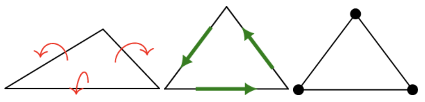
The crucial point is

\[ \nabla H^1 \subset H(\operatorname{curl}), \]

so the discrete gradients of \(w_h\) are contained in the rotation space. This makes the Kirchhoff constraint representable and removes shear locking.

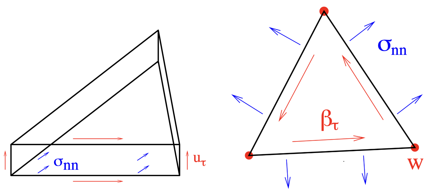
However, the gradient of the rotation, \(\nabla\beta\notin L^2\), but a distribution. To this end we apply the TDNNS method by introducing the bending moment

\[ \sigma = \mathbb{D}\varepsilon(\beta), \]

yielding the mixed formulation: Find \((w,\beta,\sigma)\) such that for all \((v,\delta,\tau)\)

\[ \int_\Omega \mathbb{D}^{-1}\sigma:\tau\,dx - \langle \tau,\nabla\beta\rangle = 0, \]

\[ -\langle \sigma,\nabla\delta\rangle - \frac{\kappa G}{t^2}\int_\Omega (\nabla w-\beta)\cdot(\nabla v-\delta)\,dx = -\int_\Omega f v\,dx. \]

The TDNNS duality pairing

\[\langle \sigma,\nabla\beta\rangle = \sum_{T}\left(\int_T\sigma:\nabla\beta\,dx - \int_{\partial T}\sigma_{nn}\beta_n\,ds\right)\]

is implemented by element terms and boundary terms involving the normal-normal component of \(\sigma\).

def SolveReissnerMindlinTDNNS(mesh, order=1, thickness=0.1, draw=False):
    fesW = H1(mesh, order=order, dirichlet="circ")
    fesB = HCurl(mesh, order=order - 1, dirichlet="circ")
    fesS = HDivDiv(mesh, order=order - 1)
    fes = fesW * fesB * fesS

    (w, beta, sigma), (v, delta, tau) = fes.TnT()
    n = specialcf.normal(2)

    a = BilinearForm(fes, symmetric=True)
    a += (
        InnerProduct(DMatInv(sigma), tau)
        - InnerProduct(tau, Grad(beta))
        - InnerProduct(sigma, Grad(delta))
    ) * dx
    a += (sigma[n, n] * delta * n + tau[n, n] * beta * n) * dx(element_boundary=True)
    a += -kappa * G / thickness**2 * (Grad(w) - beta) * (Grad(v) - delta) * dx
    a.Assemble()

    f = LinearForm(-fz * v * dx).Assemble()
    gf_solution = GridFunction(fes)
    gf_solution.vec.data = a.mat.Inverse(fes.FreeDofs(), inverse="umfpack") * f.vec

    gf_w, gf_beta, gf_sigma = gf_solution.components
    if draw:
        Draw(gf_w, mesh, "w_tdnns", deformation=True, euler_angles=[-60, 5, 30])
    return gf_w, fes

gf_w_tdnns, fes_tdnns = SolveReissnerMindlinTDNNS(mesh, order=1, thickness=0.1, draw=True);

A quick test that the TDNNS method does not suffer from shear locking:

def relative_l2_error(gf_w, mesh, thickness):
    w_ex = ExactSolution(thickness)
    return sqrt(Integrate((gf_w - w_ex) ** 2, mesh)) / sqrt(Integrate(w_ex**2, mesh))

for thickness in [1, 0.1, 0.01, 0.001, 0.0001]:
    mesh = GenerateMesh(order=2, maxh=0.5)
    gf_w, fes = SolveReissnerMindlinTDNNS(mesh, order=1, thickness=thickness)
    err = relative_l2_error(gf_w, mesh, thickness)
    print(f"t={thickness:7g}, ndof={fes.ndof:4d}, rel L2 err={err:.3e}")

t=      1, ndof= 821, rel L2 err=1.065e-01
t=    0.1, ndof= 821, rel L2 err=1.311e-01
t=   0.01, ndof= 821, rel L2 err=1.314e-01
t=  0.001, ndof= 821, rel L2 err=1.314e-01
t= 0.0001, ndof= 821, rel L2 err=1.314e-01

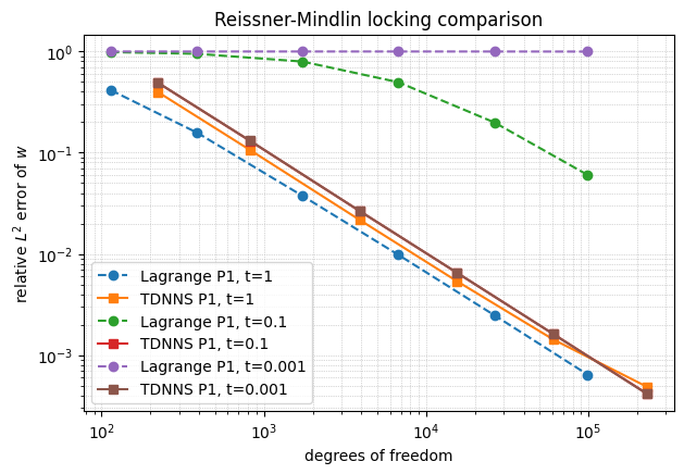
9.4. Locking comparison

The following plot compares the equal-order Lagrange discretization with the TDNNS discretization for decreasing mesh size. The displacement space has order one in both methods. For small thickness, the Lagrange method becomes too stiff on practical meshes, while the TDNNS method keeps the Kirchhoff constraint compatible with the discrete spaces.

import matplotlib.pyplot as plt


def compute_locking_data(solver, thicknesses, maxhs, order):
    data = {}
    for thickness in thicknesses:
        values = []
        for maxh in maxhs:
            mesh = GenerateMesh(order=2, maxh=maxh)
            gf_w, fes = solver(mesh, order=order, thickness=thickness)
            err = relative_l2_error(gf_w, mesh, thickness)
            values.append((fes.ndof, float(err)))
        data[thickness] = values
    return data


thicknesses = [1, 0.1, 0.001]
maxhs = [1.0, 0.5, 0.25, 0.125, 0.125 / 2, 0.125 / 4]

with TaskManager():
    standard_data = compute_locking_data(
        SolveReissnerMindlinLagrange,
        thicknesses=thicknesses,
        maxhs=maxhs,
        order=1,
    )
    tdnns_data = compute_locking_data(
        SolveReissnerMindlinTDNNS,
        thicknesses=thicknesses,
        maxhs=maxhs,
        order=1,
    )

plt.figure(figsize=(7, 4.5))
for thickness in thicknesses:
    ndof, err = zip(*standard_data[thickness])
    plt.loglog(ndof, err, "o--", label=f"Lagrange P1, t={thickness:g}")

    ndof, err = zip(*tdnns_data[thickness])
    plt.loglog(ndof, err, "s-", label=f"TDNNS P1, t={thickness:g}")

plt.xlabel("degrees of freedom")
plt.ylabel("relative $L^2$ error of $w$")
plt.title("Reissner-Mindlin locking comparison")
plt.grid(True, which="both", ls=":", lw=0.5)
plt.legend()
plt.show()

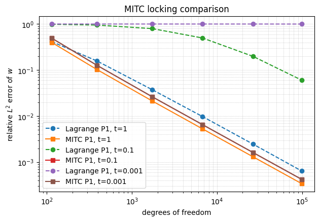
9.5. Remark: relation to MITC

Another classical way to avoid shear locking in Reissner-Mindlin plates is the MITC idea: do not use the raw shear strain

\[ \nabla w - \beta \]

directly in the shear energy, but replace it by a suitable interpolated shear strain. In the mixed finite element language, this can be interpreted as projecting/interpolating the shear strain into a compatible \(H(\operatorname{curl})\)-type space. This is closely related in spirit to the TDNNS construction: the thin limit is treated by choosing a shear/rotation representation that is compatible with gradients of the displacement.

The idea is to introduce an interpolation (reduction) operator \(\boldsymbol{R}:[H^1_0(\Omega)]^2\to H(\text{curl})\). Spaces are chosen according to [Brezzi, Fortin and Stenberg. Error analysis of mixed-interpolated elements for Reissner-Mindlin plates. Mathematical Models and Methods in Applied Sciences 1, 2 (1991), 125-151.] $\(\frac{t^3}{12}\int_{\Omega} 2\mu\, \varepsilon(\beta):\varepsilon(\delta\beta) + \lambda\, \text{div}(\beta)\text{div}(\delta\beta)\,dx + t\kappa\,G\int_{\Omega}\boldsymbol{R}(\nabla u-\beta)\cdot\boldsymbol{R}(\nabla\delta u-\delta\beta)\,dx = \int_{\Omega} f\,\delta u\,dx,\qquad \forall (\delta u,\delta\beta). \)$

The emphasis here is different. MITC modifies the shear strain field, while TDNNS changes the mixed formulation and the rotation/moment spaces so that the Kirchhoff constraint is naturally represented.

def SolveReissnerMindlinMITC(mesh, order=1, thickness=0.1, draw=False):
    fesB = VectorH1(mesh, order=order, dirichlet="circ")
    fesB.SetOrder(TRIG, order + 1 if order < 4 and order > 1 else order)
    fesB.Update()
    fesW = H1(mesh, order=order, dirichlet="circ")
    fes = fesB * fesW
    (beta, w), (delta, v) = fes.TnT()

    Gamma = HCurl(mesh, order=order, type1=True)

    a = BilinearForm(fes, symmetric=True)
    a += InnerProduct(DMat(Sym(Grad(beta))), Sym(Grad(delta))) * dx
    if order > 1:
        a += (
            kappa * G / thickness**2
            * Interpolate(grad(w) - beta, Gamma)
            * Interpolate(grad(v) - delta, Gamma)
            * dx
        )
    else:
        # lowest order needs a stabilization technique
        # the stability parameter->0 for h->0
        h = specialcf.mesh_size
        a += (
            kappa * G / (thickness**2 + h**2)
            * Interpolate(grad(w) - beta, Gamma)
            * Interpolate(grad(v) - delta, Gamma)
            * dx
        )
    a.Assemble()
    
    f = LinearForm(fz * v * dx).Assemble()

    gf_solution = GridFunction(fes)
    gf_beta, gf_w = gf_solution.components
    gf_solution.vec.data = a.mat.Inverse(fes.FreeDofs(), inverse="sparsecholesky") * f.vec
    if draw:
        Draw(gf_w, mesh, "w", deformation=True, euler_angles=[-60, 5, 30])
    return gf_w, fes


gf_w_mitc, fes_mitc = SolveReissnerMindlinMITC(mesh, order=2, thickness=0.1, draw=True);

import matplotlib.pyplot as plt


def compute_locking_data(solver, thicknesses, maxhs, order):
    data = {}
    for thickness in thicknesses:
        values = []
        for maxh in maxhs:
            mesh = GenerateMesh(order=2, maxh=maxh)
            gf_w, fes = solver(mesh, order=order, thickness=thickness)
            err = relative_l2_error(gf_w, mesh, thickness)
            values.append((fes.ndof, float(err)))
        data[thickness] = values
    return data


thicknesses = [1, 0.1, 0.001]
maxhs = [1.0, 0.5, 0.25, 0.125, 0.125 / 2, 0.125 / 4]

with TaskManager():
    standard_data = compute_locking_data(
        SolveReissnerMindlinLagrange,
        thicknesses=thicknesses,
        maxhs=maxhs,
        order=1,
    )
    mitc_data = compute_locking_data(
        SolveReissnerMindlinMITC,
        thicknesses=thicknesses,
        maxhs=maxhs,
        order=1,
    )

plt.figure(figsize=(7, 4.5))
for thickness in thicknesses:
    ndof, err = zip(*standard_data[thickness])
    plt.loglog(ndof, err, "o--", label=f"Lagrange P1, t={thickness:g}")

    ndof, err = zip(*mitc_data[thickness])
    plt.loglog(ndof, err, "s-", label=f"MITC P1, t={thickness:g}")

plt.xlabel("degrees of freedom")
plt.ylabel("relative $L^2$ error of $w$")
plt.title("MITC locking comparison")
plt.grid(True, which="both", ls=":", lw=0.5)
plt.legend()
plt.show()