Fluid-structure interaction

19. Fluid-structure interaction#

In this notebook we introduce the ingredients of a monolithic fluid-structure interaction (FSI) formulation. The aim is not yet to discuss all implementation details, but to make clear which equations live on which domain, why an Arbitrary Lagrangian Eulerian (ALE) formulation is useful for the fluid, and how the interface conditions enter the weak form. Afterwards, two discretizations of the fluid part are presented:

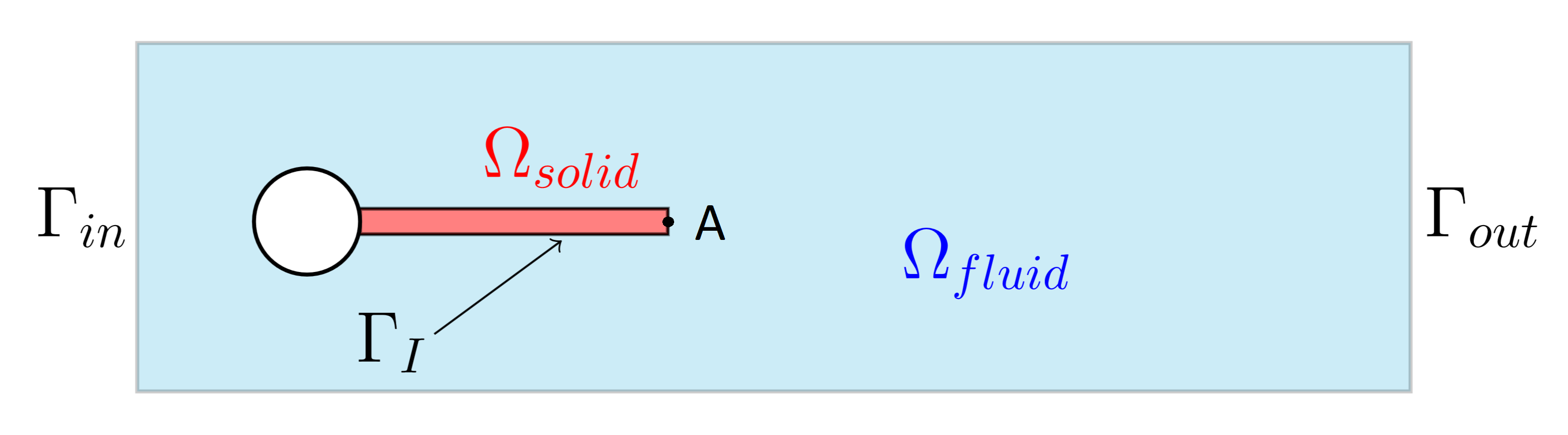
We distinguish three fields:

field	domain	role
\(u_f, p_f\)	fluid	fluid velocity and pressure
\(d_s, u_s=\dot d_s\)	solid	solid displacement and solid velocity
\(d_m, w_m=\dot d_m\)	fluid mesh	artificial mesh displacement and mesh velocity for ALE

Equations on fluid and solid

The Navier-Stokes equations with symmetric stress, velocity \(u_f\), and pressure \(p_f\) are considered for the fluid part on the current fluid domain:

\[\begin{split} \begin{align*} &\rho_f\frac{\partial u_f}{\partial t} + \rho_f(u_f\cdot \nabla)u_f -\rho_f\nu_f \mathrm{div}(\nabla u_f^\top+\nabla u_f) + \nabla p_f = f_f,\\ &\mathrm{div}(u_f) = 0. \end{align*} \end{split}\]

Here \(\rho_f\) is the fluid density and \(\nu_f\) is the kinematic viscosity. For the solid we use the elastic wave equation in Lagrangian coordinates with displacement \(d_s\) and first Piola-Kirchhoff stress tensor \(P_s=F_s\Sigma_s\):

\[ \begin{align*} \rho_s\frac{\partial^2 d_s}{\partial t^2} - \mathrm{div}(F_s\Sigma_s) = g_s. \end{align*} \]

We consider a St. Venant-Kirchhoff material law

\[ \begin{align*} \Sigma_s = 2\mu_s E_s + \lambda_s \mathrm{tr}(E_s)I,\quad F_s = I + \nabla d_s,\quad E_s=\frac{1}{2}(F_s^\top F_s-I), \end{align*} \]

with \(\mu_s\), \(\lambda_s\) the Lamé parameters.

Navier-Stokes in ALE (Arbitrary Lagrangian Eulerian) formulation

The Navier-Stokes equations are given in Eulerian form, whereas the elasticity problem is formulated in Lagrangian coordinates. To couple the two descriptions on one reference configuration, we use an Arbitrary Lagrangian Eulerian form (short ALE) for the fluid part, see e.g. [Donea, Huerta, Ponthot, Rodríguez-Ferran. Arbitrary Lagrangian-Eulerian Methods. In: Encyclopedia of Computational Mechanics, 2004].

We work on a fixed reference fluid domain \(\hat\Omega_f\). Let \(\Phi(\hat x,t)=\hat x+d_m(\hat x,t)\) describe the movement of the fluid mesh, where \(d_m\) is the mesh displacement. The current and reference fluid velocities are related by

\[ \begin{align*} u_f\circ\Phi=\hat{u}_f. \end{align*} \]

The spatial chain rule gives

\[ \begin{align*} \nabla_xu_f\circ\Phi = \nabla_{\hat{x}}\hat{u}_fF_m^{-1}, \end{align*} \]

where \(F_m=\nabla\Phi\) denotes the mesh deformation gradient. For the time derivative at fixed Eulerian position one obtains

\[ \begin{align*} \frac{\partial u_f}{\partial t}\circ\Phi = \frac{\partial\hat{u}_f}{\partial t} - (\nabla_{\hat{x}}\hat{u}_fF_m^{-1})\,w_m, \qquad w_m=\frac{\partial \Phi}{\partial t}=\dot d_m. \end{align*} \]

Thus the convective velocity in ALE coordinates is the relative velocity \(\hat u_f-w_m\). Applying the transformation theorem introduces the Jacobian \(J_m=\det(F_m)\). The ALE Navier-Stokes equations can then be written in weak form as

\[\begin{split} \begin{align*} &\int_{\hat\Omega_f}J_m\Big(\rho_f\frac{\partial \hat{u}_f}{\partial t}\cdot\hat{v} +\rho_f(\nabla_{\hat x}\hat{u}_fF_m^{-1})(\hat{u}_f-w_m)\cdot\hat{v} +2\rho_f\nu_f \mathrm{sym}(\nabla_{\hat x}\hat{u}_fF_m^{-1}):\mathrm{sym}(\nabla_{\hat x}\hat{v}F_m^{-1}) -\mathrm{tr}(\nabla_{\hat x}\hat{v}F_m^{-1})p_f\Big)\,d\hat x = 0&&\qquad \forall \hat{v},\\ &\int_{\hat\Omega_f}J_m\,\mathrm{tr}(\nabla_{\hat x}\hat{u}_fF_m^{-1})q\,d\hat x = 0&&\qquad \forall q. \end{align*} \end{split}\]

Elastic wave equation as first order system

The elastic wave equation does not have to be transformed, since it is already stated in Lagrangian coordinates. We rewrite it as a first order system in time by introducing the solid velocity \(u_s=\dot{d}_s\). The variational formulation is therefore given by

\[\begin{split} \begin{align*} & \int_{\Omega_s}\frac{\partial d_s}{\partial t}\cdot v \,dX = \int_{\Omega_s}u_s\cdot v\,dX &&\qquad \forall v,\\ &\int_{\Omega_s}\rho_s\frac{\partial u_s}{\partial t}\cdot w+(F_s\Sigma_s):\nabla w\,dX = 0&&\qquad \forall w. \end{align*} \end{split}\]

Interface conditions The interface conditions for fluid-structure interaction have to be considered before we can couple the equations. On the physical interface the fluid velocity equals the solid velocity, while the ALE mesh displacement follows the solid displacement:

\[ \begin{align*} u_f = u_s=\dot d_s, \qquad d_m=d_s \qquad \text{on } \Gamma_I. \end{align*} \]

The dynamic condition is balance of traction. In a reference formulation this can be expressed schematically as

\[ \begin{align*} \int_{\Gamma_I} \hat\sigma_f \hat n_f\cdot \hat v_f\,d\hat s + \int_{\Gamma_I} P_s n_s\cdot w_s\,dS = 0 \end{align*} \]

for compatible test functions on the interface. In a monolithic conforming discretization, the interface velocity is represented by the same unknown on both sides. The two interface traction terms then cancel in the summed weak form and the traction balance is imposed naturally.

Deformation extension into fluid domain

The last important ingredient is the deformation extension. The mesh displacement \(d_m\) and mesh velocity \(w_m=\dot d_m\) in the ALE Navier-Stokes equations are artificial. They have to be constructed from the solid displacement on the interface.

A simple approach is to solve a Poisson problem on the fluid domain with \(d_m=d_s\) on the interface and homogeneous Dirichlet conditions on the fixed outer boundary. This is often sufficient for small deformations, but it may lead to poor mesh quality or even inverted elements for larger motions.

A more robust approach is to solve an auxiliary nonlinear elasticity problem for the fluid mesh. One usually increases the artificial stiffness in sensitive regions and penalizes volume compression, so that elements close to the moving structure do not collapse. In the implementation notebooks below this is realized by a spatially dependent stiffness function \(h(x)\) and a volume-penalizing mesh energy.

The extension problem is not a physical model for the solid. It only defines the ALE map in the fluid domain. If the extension is solved together with the physical unknowns in a monolithic system, its influence on the physical solid equations is scaled by a small parameter.