13. Implementation of High Order Finite Elements

A starting point to NGSolve-programming, used in my finite element class.

Get repository from github

• Finite elements implement the basis functions: myhoelement.hpp and myhoelement.cpp

• Finite element spaces implement the enumeration of degrees of freedom, and creation of elements: myhofespace.hpp and myhofespace.cpp

See Dissertation Sabine Zaglmayr , page 60 ff

Basis functions are based on Legendre polynomials \(P_i\):

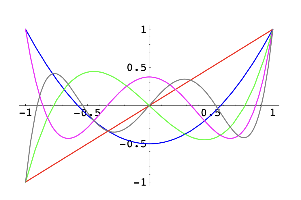
and on Integrated Legendre polynomials \(L_{i+1}(x) := \int_{-1}^x P_i(s) ds\)

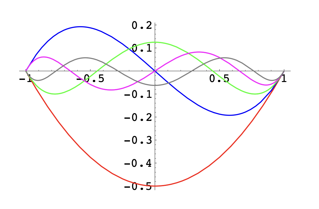
The integrated Legendre polynomials vanish at the boundary, and thus are useful for bubble functions.

Basis functions for the segment:

Vertex basis functions:

\[ \varphi_i(x) = \lambda_i(x) \qquad 0 \leq i < 2 \]

Inner basis functions (on edges), where \(\lambda_s\) and \(\lambda_e\) are barycentric for the start-point, and end-point of the edge:

\[ \varphi^E_i(x) = L_{i+2}(\lambda_e - \lambda_s) \qquad 0 \leq i < p-1 \]

Basis functions for the triangle:

Vertex basis functions:

\[ \varphi_i(x) = \lambda_i(x) \qquad 0 \leq i < 3 \]

Edge-based basis functions on the edge E, where \(\lambda_s\) and \(\lambda_e\) are barycentric for the start-point, and end-point of the edge:

\[ \varphi^E_i(x,y) = L_{i+2}\left(\frac{\lambda_e - \lambda_s}{\lambda_e + \lambda_s} \right) (\lambda_e+\lambda_s)^{i+2} \qquad 0 \leq i < p-1 \]

• on the edge E, there is \(\lambda_s + \lambda_e = 1\), and thus the function corresponds with the integrated Legendre polynomials \(L_{i+2}\).

• on the other two edges, either \(\lambda_s = 0\) or \(\lambda_e = 0\). Thus, the argument of \(L_{i+2}\) is either \(-1\), or \(+1\). Thus, the shape function vanishes at the other two edges.

• The first factor is a rational function. Then we multiply with a polynomial, such that the denominator cancels out. Thus the basis functions are polynomials.

Inner basis functions (on the triangular face F):

\[ \varphi^F_{i,j}(x,y) = L_{i+2}\left(\frac{\lambda_0 - \lambda_1}{\lambda_0 + \lambda_1} \right) (\lambda_0+\lambda_1)^{i+2} P_j (2 \lambda_2 -1) \lambda_2 \qquad 0 \leq i,j \text{ and } i+j \leq p-3 \]

from ngsolve import *
from ngsolve.webgui import Draw
from myhofe import MyHighOrderFESpace

mesh = Mesh(unit_square.GenerateMesh(maxh=0.2, quad_dominated=False))

Loading myhofe library

We can now create an instance of our own finite element space:

fes = MyHighOrderFESpace(mesh, order=4, dirichlet="left|bottom|top")

and use it within NGSolve such as the builtin finite element spaces:

print ("ndof = ", fes.ndof)

ndof =  489

gfu = GridFunction(fes)
gfu.Set(x*x*y*y)

Draw (gfu)
Draw (grad(gfu)[0], mesh);

and solve the standard problem:

u,v = fes.TnT()
a = BilinearForm(grad(u)*grad(v)*dx).Assemble()
f = LinearForm(10*v*dx).Assemble()
gfu.vec.data = a.mat.Inverse(fes.FreeDofs())*f.vec
Draw (gfu, order=3);

errlist = []
for p in range(1,13):
    fes = MyHighOrderFESpace(mesh, order=p)
    func = sin(pi*x)*sin(pi*y)
    gfu = GridFunction(fes)
    gfu.Set(func)
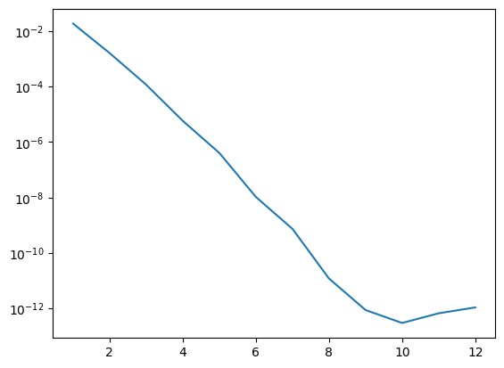
    err = sqrt(Integrate( (func-gfu)**2, mesh, order=5+2*p))
    errlist.append((p,err))
print (errlist)

[(1, 0.018470559015394374), (2, 0.0016028677378609774), (3, 0.00011616801306622328), (4, 5.803815226396687e-06), (5, 4.056875365934112e-07), (6, 1.048343926954013e-08), (7, 7.453642469120944e-10), (8, 1.2057545365774509e-11), (9, 8.830930833275869e-13), (10, 3.0215817442800976e-13), (11, 6.757271820168648e-13), (12, 1.0997447299037109e-12)]

import matplotlib.pyplot as plt
n,err = zip(*errlist)
plt.yscale('log')
plt.plot(n,err);

Exercises:

Extend MyHighOrderFESpace by high order quadrilateral elements.