3. Hybrid Discontinuous Galerkin (HDG) methods for elliptic equations

\(\DeclareMathOperator{\opdiv}{div}\)

The HDG method involves discontinuous polynomials on elements, and additional polynomials on the edges (or faces, in 3D).

We start from the Poisson equation

\[ -\Delta u = f \]

multiply by discontinuous test functions, integrate by parts on every element:

\[ \sum_T \int_T \nabla u \nabla v - \int_{\partial T} \frac{\partial u}{\partial n} v = \int_\Omega f v \]

Since the normal-derivatives are continuous from element to element, we can smuggle in a single-valued test-function \(\widehat v\) on every edge:

\[ \sum_T \int_T \nabla u \nabla v - \int_{\partial T} \frac{\partial u}{\partial n} (v-\widehat{v}) = \int_\Omega f v \]

This is a non-symmetric bilinear-form for the self-adjoint Poisson operator, what we don’t like. For the true solution \(u\), the solution on the elements restricted to the edges is the same as the solution restricted to the edges, we are adding a zero term:

\[ \sum_T \int_T \nabla u \nabla v - \int_{\partial T} \frac{\partial u}{\partial n} (v-\widehat{v}) - \int_{\partial T} \frac{\partial v}{\partial n} (u-\widehat{u}) = \int_\Omega f v \]

This form may not be coercive, and we have to add a stabilization term:

\[ \sum_T \int_T \nabla u \nabla v - \int_{\partial T} \frac{\partial u}{\partial n} (v-\widehat{v}) - \int_{\partial T} \frac{\partial v}{\partial n} (u-\widehat{u}) + \int_{\partial T} \frac{\alpha p^2}{h} (u-\widehat{u}) (v-\widehat{v}) = \int_\Omega f v \]

Here, \(h\) is the element-size, \(p\) the polynomial order, and \(\alpha\) a sufficiently large stabilization parameter (typically 3 in 2D and 10 in 3D). This ‘sufficiently large’ condition is a drawback of the so called interior penalty version of DG/HDG, but there exist more sophisticated, robust versions.

3.1. Projected jumps:

Lehrenfeld ‘10, Lehrenfeld+JS ‘16

By inserting an \(L_2(E)\)-projector into the jump-term, we can reduce the polynomial order of the facet-variable by one order, and maintain the same order of convergence.

\[ \sum_T \int_T \nabla u \nabla v - \int_{\partial T} \frac{\partial u}{\partial n} (v-\widehat{v}) - \int_{\partial T} \frac{\partial v}{\partial n} (u-\widehat{u}) + \int_{\partial T} \frac{\alpha p^2}{h} (P u-\widehat{u}) (P v-\widehat{v}) = \int_\Omega f v \]

Implementation:

• use an \(L_2\)-orthogonal basis on the facet

• associate highest order basis functions to elements, not to faces

from ngsolve import *
from ngsolve.webgui import Draw
mesh = Mesh(unit_square.GenerateMesh(maxh=0.1))

order = 3
fes1 = L2(mesh, order=order)
fes2 = FacetFESpace(mesh, order=order, dirichlet="left|bottom", 
                    highest_order_dc=False)
fes = fes1 * fes2

u,uhat = fes.TrialFunction()
v,vhat = fes.TestFunction()

h = specialcf.mesh_size
n = specialcf.normal(2)
alpha = 3
dS = dx(element_vb=BND)

a = BilinearForm(fes, condense=True)
a += grad(u)*grad(v)*dx
a += (-n*grad(u)*(v-vhat)-n*grad(v)*(u-uhat))*dS
a += alpha*(order+1)**2/h*(u-uhat)*(v-vhat)*dS

f = LinearForm(fes)
f += 1*v*dx

a.Assemble()
f.Assemble();

print ("ndof: ", fes.ndof)
print ("non-zero(A):", a.mat.nze)
print ("non-zero(Inv):", a.mat.Inverse(fes.FreeDofs(a.condense), "sparsecholesky").nze)

ndof:  3760
non-zero(A): 27920
non-zero(Inv): 38326

gfu = GridFunction(fes)
solvers.BVP(bf=a, lf=f, gf=gfu)
Draw (gfu.components[0]);

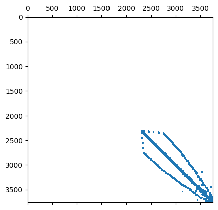
The coupling of element-variables happens only through the facet variables:

import scipy.sparse as sp
import matplotlib.pyplot as plt
scipymat = sp.csr_matrix(a.mat.CSR())
plt.spy(scipymat, precision=1e-10, markersize=1);

degrees of freedom, non-zero matrix entries and entries of the inverse for \(p=3\):

condense	projection	ndof	nze-mat	nze-inv
False	False	3760	106120	75572
False	True	4085	108395	67821
True	False	3760	27920	38326
True	True	4085	15705	21735